Evaluation Report - claude

📝 ABC

42/45 (93.3%)

📋 Task Description

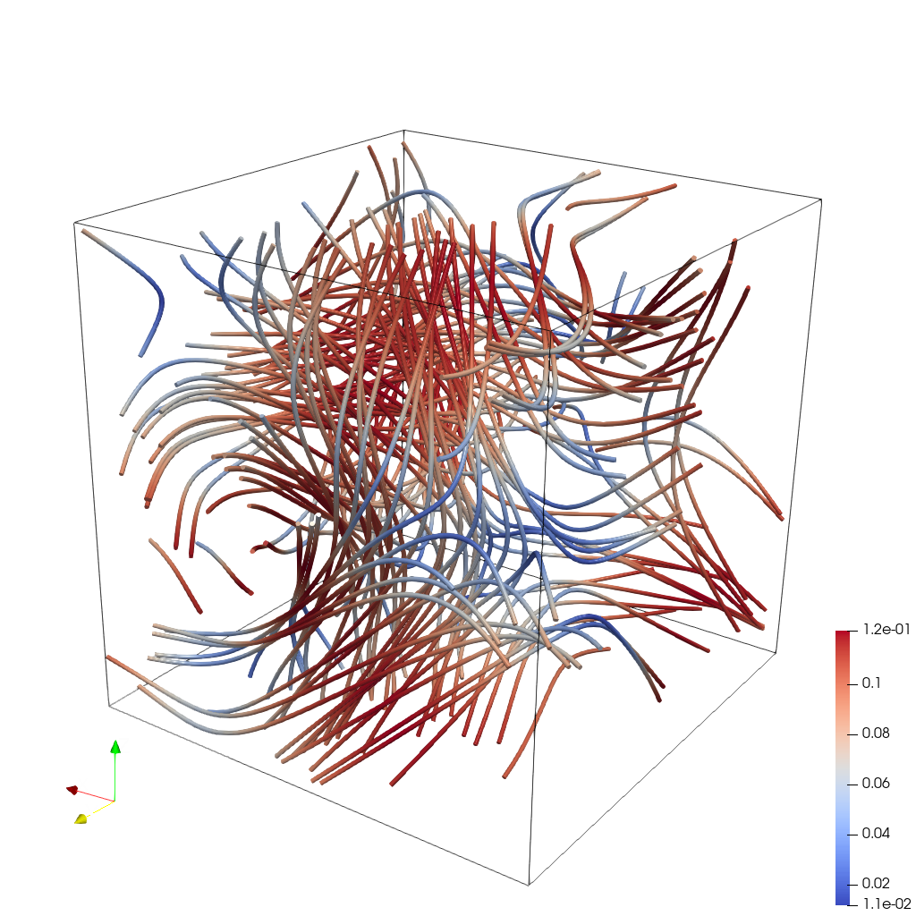
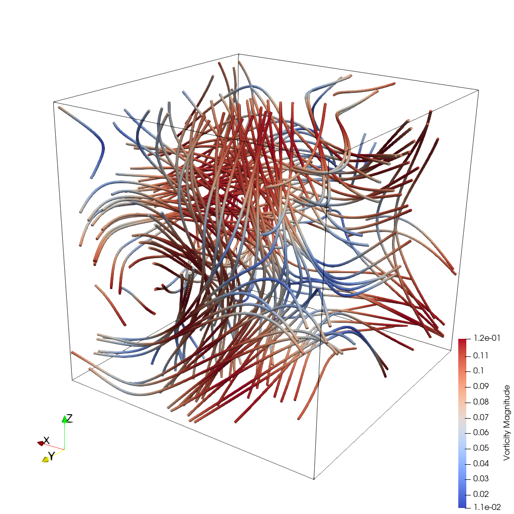
Load the ABC (Arnold-Beltrami-Childress) flow vector field from "ABC/data/ABC_128x128x128_float32_scalar3.raw", the information about this dataset: ABC Flow (Vector) Data Scalar Type: float Data Byte Order: Little Endian Data Extent: 128x128x128 Number of Scalar Components: 3 Data loading is very important, make sure you correctly load the dataset according to their features. Create streamlines using a "Stream Tracer" filter with "Point Cloud" seed type. Set the seed center to [73.77, 63.25, 71.65], with 150 seed points and a radius of 75.0. Set integration direction to "BOTH" and maximum streamline length to 150.0. Add a "Tube" filter on the stream tracer to enhance visualization. Set tube radius to 0.57 with 12 sides. Color the tubes by Vorticity magnitude using the 'Cool to Warm (Diverging)' colormap. Show the dataset bounding box as an outline. Use a white background. Render at 1024x1024. Set the viewpoint parameters as: [-150.99, 391.75, 219.64] to position; [32.38, 120.41, 81.63] to focal point; [0.23, -0.31, 0.92] to camera up direction. Save the visualization image as "ABC/results/{agent_mode}/ABC.png". (Optional, but must save if use paraview) Save the paraview state as "ABC/results/{agent_mode}/ABC.pvsm". (Optional, but must save if use python script) Save the python script as "ABC/results/{agent_mode}/ABC.py". Do not save any other files, and always save the visualization image.

🖼️ Visualization Comparison

Ground Truth

Agent Result

📏 Vision Evaluation Rubrics

Score Summary

Total Score

29/30

Goals

3

Points/Goal

10

Goal 1

10/10

Criterion: Streamline Density: Are the streamline tubes densely distributed throughout the volume, similar to the ground truth?

Judge's Assessment: The result shows a very similar number of tube streamlines and overall spatial distribution to the ground truth: a dense central bundle with many arcs extending toward the box faces/edges. Coverage throughout the volume and the balance of streamline lengths match closely, with no obvious missing regions or large over/under-seeding compared to the ground truth.

Goal 2

9/10

Criterion: Color Mapping: Are the tubes colored by vorticity magnitude using a blue-white-red diverging colormap, with a similar color distribution as the ground truth?

Judge's Assessment: The tubes use a blue–white–red diverging scheme consistent with Cool-to-Warm and are labeled as vorticity magnitude. The overall color distribution (many warm reds/oranges in the central region and scattered cool blues on peripheral arcs) matches the ground truth closely. Minor differences appear in exact saturation/contrast and the colorbar styling/labeling, but the mapping looks essentially correct.

Goal 3

10/10

Criterion: Tube Appearance: Do the streamline tubes have a similar thickness and smooth appearance as the ground truth?

Judge's Assessment: Tube thickness and smoothness appear virtually identical to the ground truth: consistent radius, rounded tube appearance, and similar surface shading/specular response. No noticeable faceting beyond what is expected, and the visual weight of the tubes relative to the outline box matches well.

Overall Assessment

Overall the result is an excellent match to the ground truth. Streamline density and tube rendering closely replicate the expected visualization, and the diverging vorticity-magnitude coloring is correct with only minor, largely cosmetic differences in color intensity/colorbar presentation.

📊 Detailed Metrics

Visualization Quality

29/30

Output Generation

5/5

Efficiency

8/10

Completed in 137.44 seconds (good)

PSNR

25.21 dB

SSIM

0.9821

LPIPS

0.0330

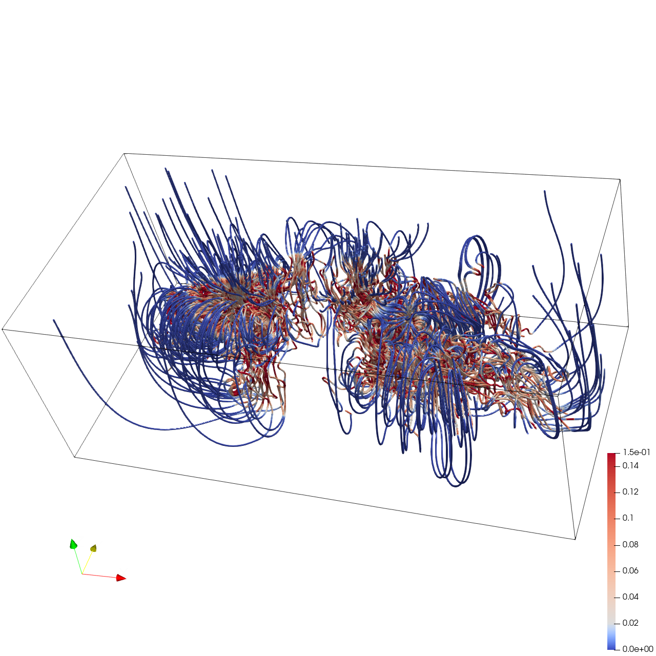
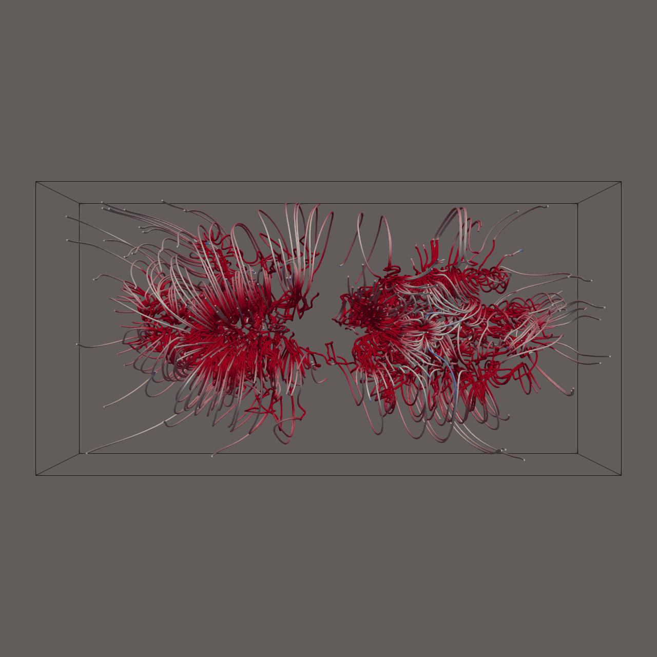
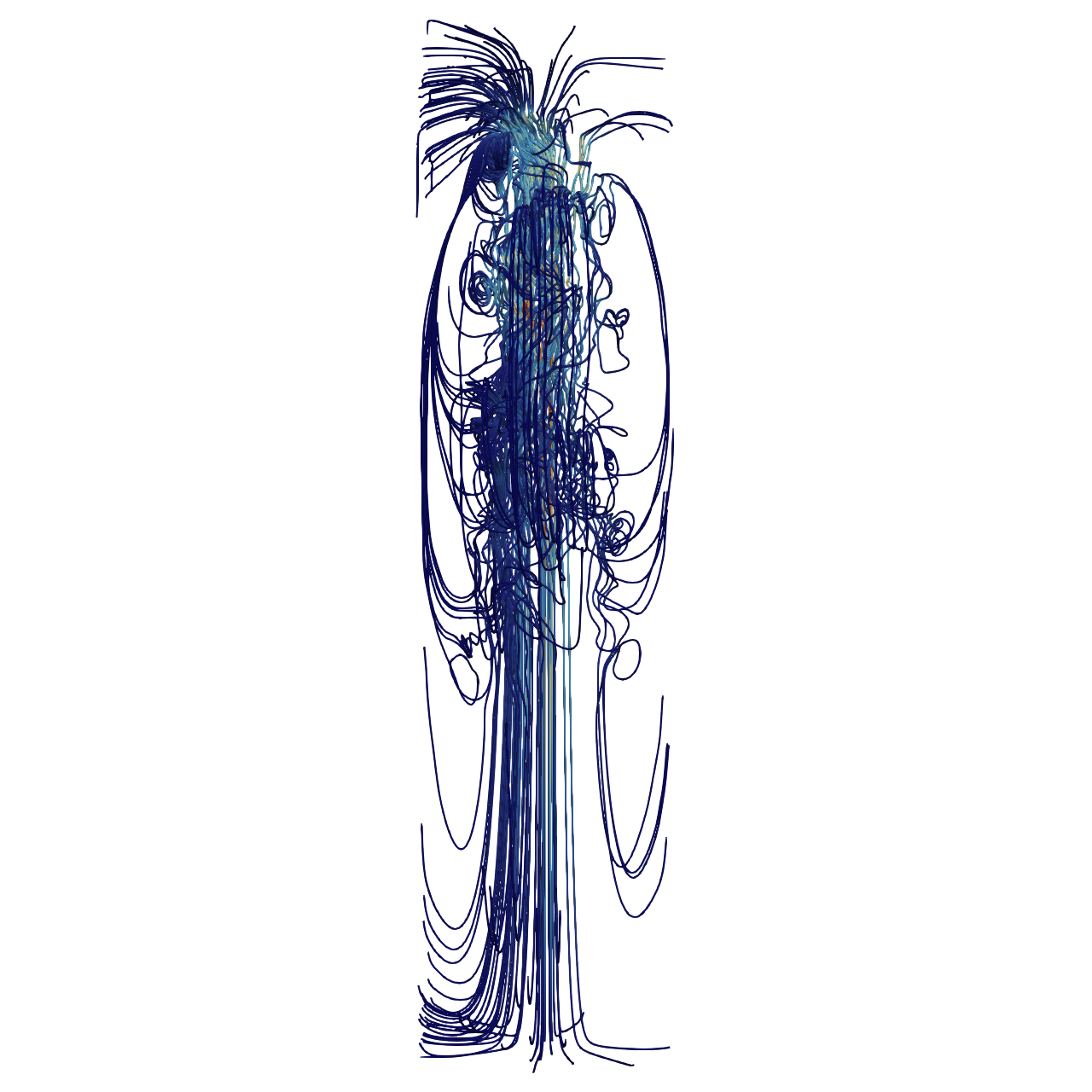
📝 Bernard

40/45 (88.9%)

📋 Task Description

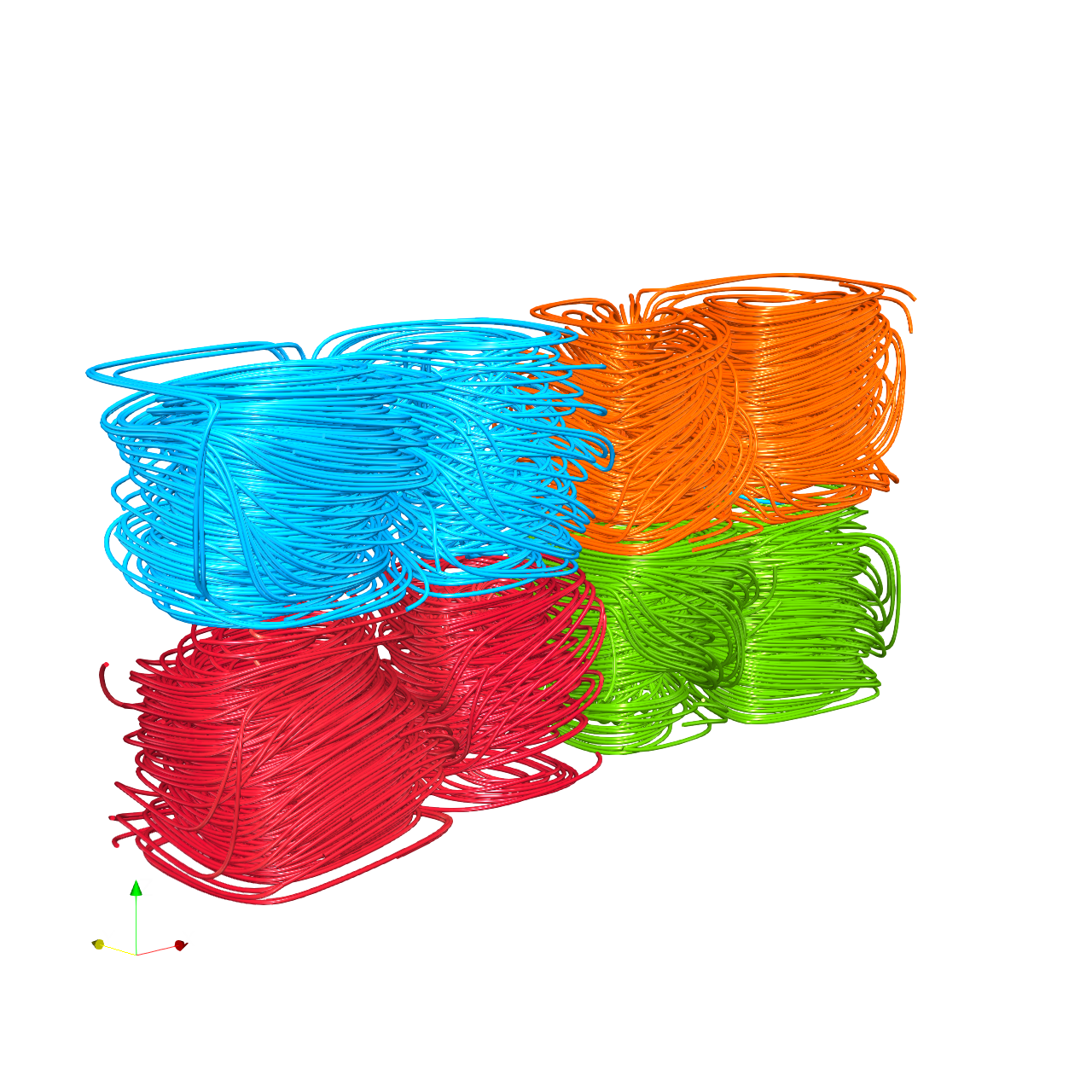
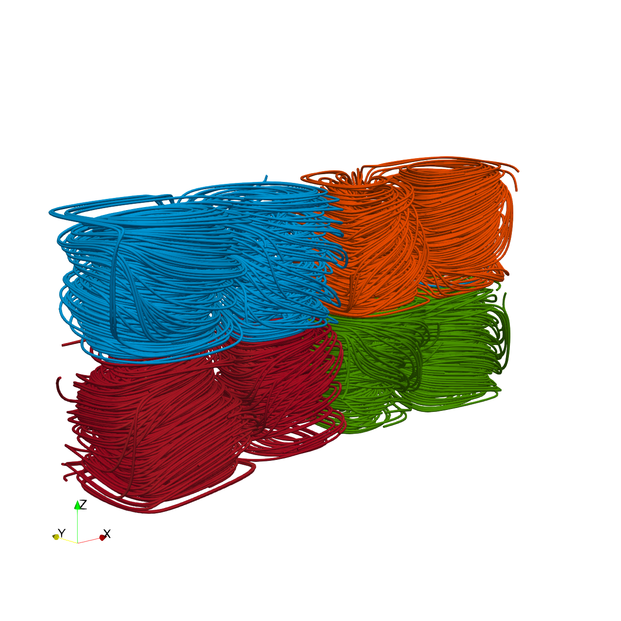
Load the Rayleigh-Benard convection vector field from "Bernard/data/Bernard_128x32x64_float32_scalar3.raw", the information about this dataset: Rayleigh-Benard Convection (Vector) Data Scalar Type: float Data Byte Order: Little Endian Data Extent: 128x32x64 Number of Scalar Components: 3 Data loading is very important, make sure you correctly load the dataset according to their features. Create four streamline sets using "Stream Tracer" filters with "Point Cloud" seed type, each with 100 seed points and radius 12.7: - Streamline 1: Seed center at [30.69, 14.61, 47.99]. Apply a "Tube" filter (radius 0.3, 12 sides). Color with solid blue (RGB: 0.0, 0.67, 1.0). - Streamline 2: Seed center at [91.10, 14.65, 45.70]. Apply a "Tube" filter (radius 0.3, 12 sides). Color with solid orange (RGB: 1.0, 0.33, 0.0). - Streamline 3: Seed center at [31.87, 12.76, 15.89]. Apply a "Tube" filter (radius 0.3, 12 sides). Color by velocity magnitude using the 'Cool to Warm (Diverging)' colormap. - Streamline 4: Seed center at [92.09, 10.50, 15.32]. Apply a "Tube" filter (radius 0.3, 12 sides). Color with solid green (RGB: 0.33, 0.67, 0.0). In the pipeline browser panel, hide all stream tracers and only show the tube filters. Use a white background. Render at 1280x1280. Do not show a color bar. Set the viewpoint parameters as: [-81.99, -141.45, 89.86] to position; [65.58, 26.29, 28.48] to focal point; [0.18, 0.20, 0.96] to camera up direction. Save the visualization image as "Bernard/results/{agent_mode}/Bernard.png". (Optional, but must save if use paraview) Save the paraview state as "Bernard/results/{agent_mode}/Bernard.pvsm". (Optional, but must save if use pvpython script) Save the python script as "Bernard/results/{agent_mode}/Bernard.py". Do not save any other files, and always save the visualization image.

🖼️ Visualization Comparison

Ground Truth

Agent Result

📏 Vision Evaluation Rubrics

Score Summary

Total Score

25/30

Goals

3

Points/Goal

10

Goal 1

9/10

Criterion: Streamline Grouping: Are there four visually separate streamline clusters arranged in a 2x2 grid pattern, similar to the ground truth?

Judge's Assessment: The ground truth shows four distinct streamline/tube clusters arranged in a clear 2x2 layout (blue top-left, orange top-right, red/magnitude bottom-left, green bottom-right). The result image matches this overall 2x2 grouping and separation very closely. Minor differences are limited to slight variations in spacing/overlap at the boundaries between adjacent groups, but the intended four-cluster structure is clearly preserved.

Goal 2

7/10

Criterion: Color Assignment: Are the four streamline groups colored in distinct colors (blue, orange, magnitude-mapped, and green), matching the ground truth color scheme?

Judge's Assessment: Blue (top-left), orange (top-right), and green (bottom-right) match the ground truth well. However, the bottom-left group in the result appears as a mostly uniform dark red rather than being colored by velocity magnitude with a visible Cool-to-Warm diverging gradient. In the ground truth, the magnitude-colored group presents as red-dominant but should still exhibit some perceptible colormap variation; the result looks more like a solid color than a magnitude mapping.

Goal 3

9/10

Criterion: Convection Cell Structure: Do the streamlines within each group show circular or helical looping patterns characteristic of convection cells?

Judge's Assessment: All four groups in the result exhibit the characteristic convection-cell streamline behavior: dense looping/helical trajectories with coherent swirling structures, closely matching the ground truth patterns in each quadrant. Only minor differences in streamline density/individual path shapes are visible, but the convection-cell structure is strongly consistent.

Overall Assessment

The result reproduces the main composition very well: four convection-cell streamline bundles in a 2x2 arrangement with correct camera/background and strong looping structure. The primary discrepancy is the third streamline set’s coloring: it should be velocity-magnitude mapped with a Cool-to-Warm diverging colormap, but it appears largely uniform red in the result.

📊 Detailed Metrics

Visualization Quality

25/30

Output Generation

5/5

Efficiency

10/10

Completed in 57.57 seconds (excellent)

PSNR

19.92 dB

SSIM

0.8971

LPIPS

0.0380

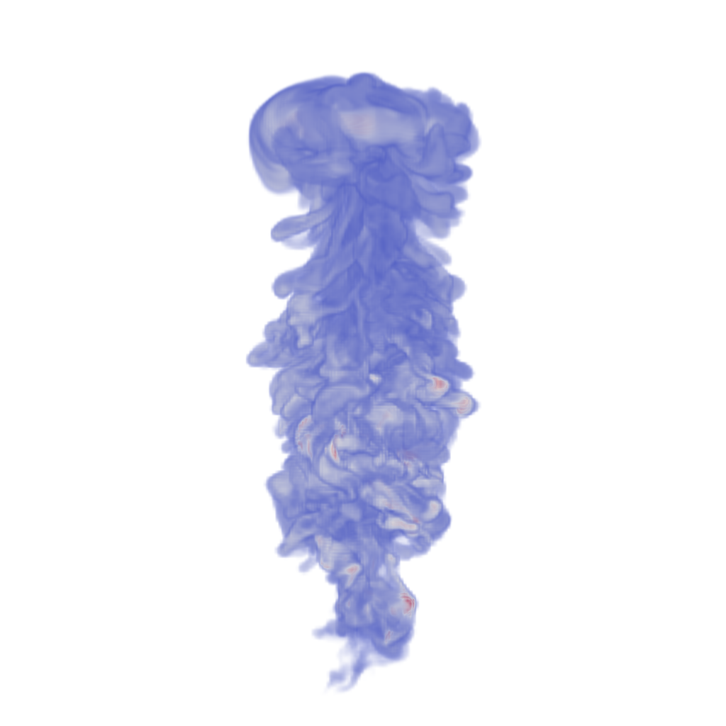
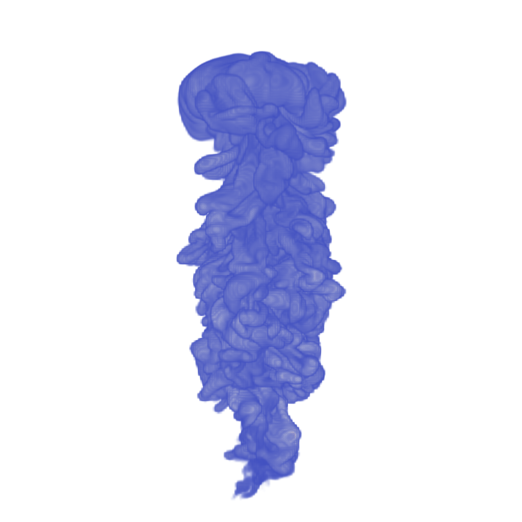
📝 argon-bubble

27/45 (60.0%)

📋 Task Description

Task: Load the Argon Bubble dataset from "argon-bubble/data/argon-bubble_128x128x256_float32.vtk". Generate a visualization image of the Argon Bubble scalar field dataset with the following visualization settings: 1) Create volume rendering 2) Set the opacity transfer function as a ramp function across values of the volumetric data, assigning opacity 0 to value 0 and assigning opacity 1 to value 1. 3) Set the color transfer function to assign a warm red color [0.71, 0.02, 0.15] to the highest value, a cool color [0.23, 0.29, 0.75] to the lowest value, and a grey color[0.87, 0.87, 0.87] to the midrange value 4) Set the viewpoint parameters as: [0, 450, 0] to position; [0, 0, -15] to focal point; [0, 0, -1] to camera up direction 5) Visualization image resolution is 1024x1024. White background. Shade turned off. Volume rendering ray casting sample distance is 0.1 6) Don't show color/scalar bar or coordinate axes. Save the visualization image as "argon-bubble/results/{agent_mode}/argon-bubble.png". (Optional, but must save if use paraview) Save the paraview state as "argon-bubble/results/{agent_mode}/argon-bubble.pvsm". (Optional, but must save if use pvpython script) Save the python script as "argon-bubble/results/{agent_mode}/argon-bubble.py". (Optional, but must save if use VTK) Save the cxx code script as "argon-bubble/results/{agent_mode}/argon-bubble.cxx" Do not save any other files, and always save the visualization image.

🖼️ Visualization Comparison

Ground Truth

Agent Result

📏 Vision Evaluation Rubrics

Score Summary

Total Score

12/30

Goals

3

Points/Goal

10

Goal 1

6/10

Criterion: Does the visualization image clearly show the regions of cool, warm, and mild regions?

Judge's Assessment: In the ground truth, the volume is predominantly cool blue with intermittent mild grey/whitish regions and a few small warm red highlights embedded inside the structure. In the result image, the volume appears almost entirely a uniform saturated blue with little to no visible midrange grey and essentially no warm red regions. The main structure is present, but the cool/warm/mild separation is not well expressed compared to the ground truth.

Goal 2

4/10

Criterion: Does the blueish region show areas with low opacity?

Judge's Assessment: The ground truth shows low-value bluish regions that are relatively translucent, letting internal layered features and faint intensity variations show through. In the result, the bluish region is much more opaque and uniform, obscuring internal variation; the overall plume looks denser and less see-through than the ground truth, indicating the low-opacity behavior for the blue range is not matched well.

Goal 3

2/10

Criterion: Does the reddish region show areas with high opacity?

Judge's Assessment: The ground truth contains small but distinct warm/red high-value spots with higher opacity (they stand out as denser bright features). The result image shows virtually no visible red regions at all, so high-opacity/high-value reddish features are not represented in a way comparable to the ground truth.

Overall Assessment

The result captures the overall plume shape and viewpoint reasonably, but the transfer functions do not match the ground truth: color mapping is dominated by a single blue tone and the opacity appears too high across most of the volume. The absence of visible red high-value features and minimal midrange grey leads to a clear mismatch for all three goals.

📊 Detailed Metrics

Visualization Quality

12/30

Output Generation

5/5

Efficiency

10/10

Completed in 56.51 seconds (excellent)

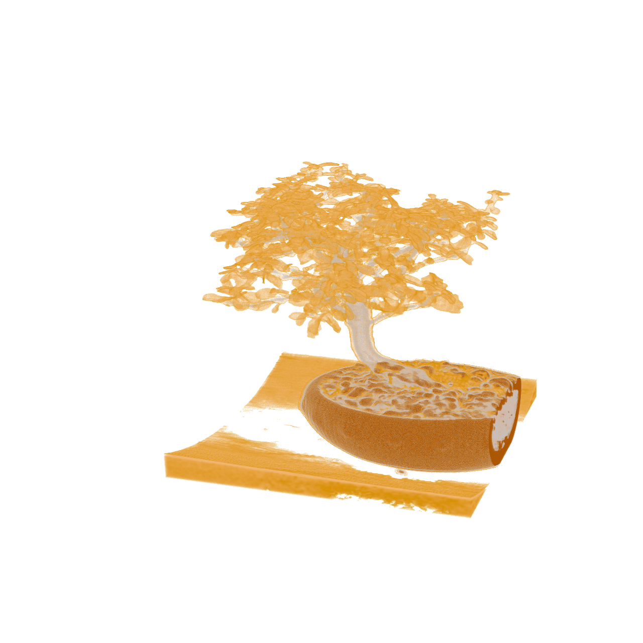
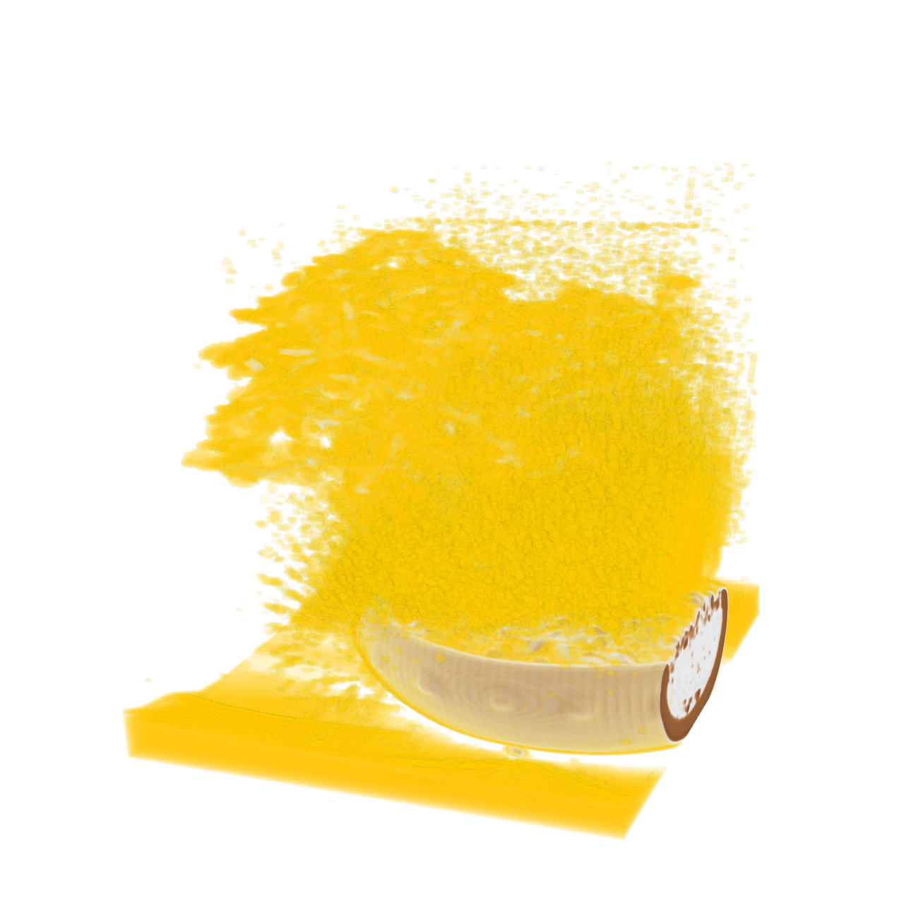
📝 bonsai

32/55 (58.2%)

📋 Task Description

Task: Load the bonsai dataset from "bonsai/data/bonsai_256x256x256_uint8.raw", the information about this dataset: Bonsai (Scalar) Data Scalar Type: unsigned char Data Byte Order: little Endian Data Spacing: 1x1x1 Data Extent: 256x256x256 Then visualize it with volume rendering, modify the transfer function and reach the visualization goal as: "A potted tree with brown pot silver branch and golden leaves." Please think step by step and make sure to fulfill all the visualization goals mentioned above. Use a white background. Render at 1280x1280. Do not show a color bar or coordinate axes. Set the viewpoint parameters as: [-765.09, 413.55, 487.84] to position; [-22.76, 153.30, 157.32] to focal point; [0.30, 0.95, -0.07] to camera up direction. Save the visualization image as "bonsai/results/{agent_mode}/bonsai.png". (Optional, but must save if use paraview) Save the paraview state as "bonsai/results/{agent_mode}/bonsai.pvsm". (Optional, but must save if use pvpython script) Save the python script as "bonsai/results/{agent_mode}/bonsai.py". Do not save any other files, and always save the visualization image.

🖼️ Visualization Comparison

Ground Truth

Agent Result

📏 Vision Evaluation Rubrics

Score Summary

Total Score

22/40

Goals

4

Points/Goal

10

Goal 1

6/10

Criterion: Overall Visualization Goal: How well does the result achieve the overall goal of showing a potted tree with the specified colors?

Judge's Assessment: The ground truth shows a clearly readable bonsai: distinct golden/orange leaves, a silver/gray trunk, and a solid brown pot. The result image captures a general tree-and-pot silhouette, but the volume rendering is dominated by a very dense, bright yellow fog that obscures the structure; the pot and trunk are much less distinct than in the ground truth.

Goal 2

4/10

Criterion: Brown Pot Visualization: Does the result show the pot portion in brown color?

Judge's Assessment: In the ground truth, the pot body is clearly brown and well-separated from the surrounding elements. In the result, the pot appears mostly pale/whitish with only a small dark-brown rim/edge visible on the right; it does not read as a predominantly brown pot.

Goal 3

5/10

Criterion: Silver Branch Visualization: Does the result show the branch/trunk portion in silver color?

Judge's Assessment: The ground truth trunk/branches are visibly silver/gray and stand out from the leaves. In the result, the trunk region is faint and largely washed out by the strong yellow volume; where visible it is light/grayish but not clearly a silver branch structure.

Goal 4

7/10

Criterion: Golden Leaves Visualization: Does the result show the leaves portion in golden color?

Judge's Assessment: Leaves in the ground truth are golden-orange with good separation of leaf clusters. In the result, the canopy is strongly golden/yellow, matching the intended hue, but it is overly opaque/noisy and lacks the leaf-structure clarity seen in the ground truth.

Overall Assessment

The result broadly matches the intended color theme for the foliage (golden) but fails to match the ground truth’s balanced transfer function that preserves clear structure. The pot is not convincingly brown and the silver trunk/branches are largely obscured by an overly dense yellow rendering.

📊 Detailed Metrics

Visualization Quality

22/40

Output Generation

5/5

Efficiency

5/10

Completed in 414.50 seconds (very slow)

PSNR

17.39 dB

SSIM

0.8823

LPIPS

0.1783

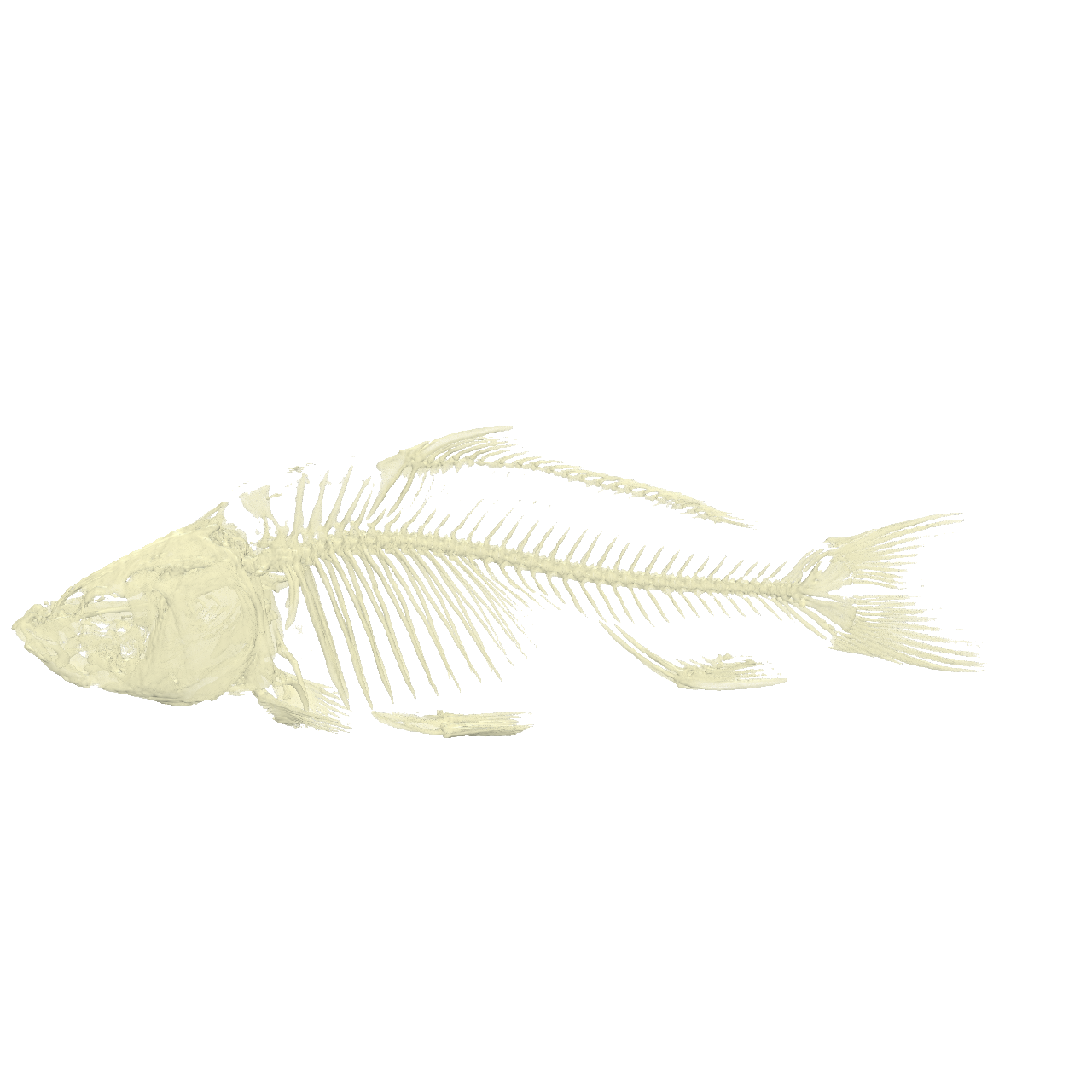
📝 carp

46/65 (70.8%)

📋 Task Description

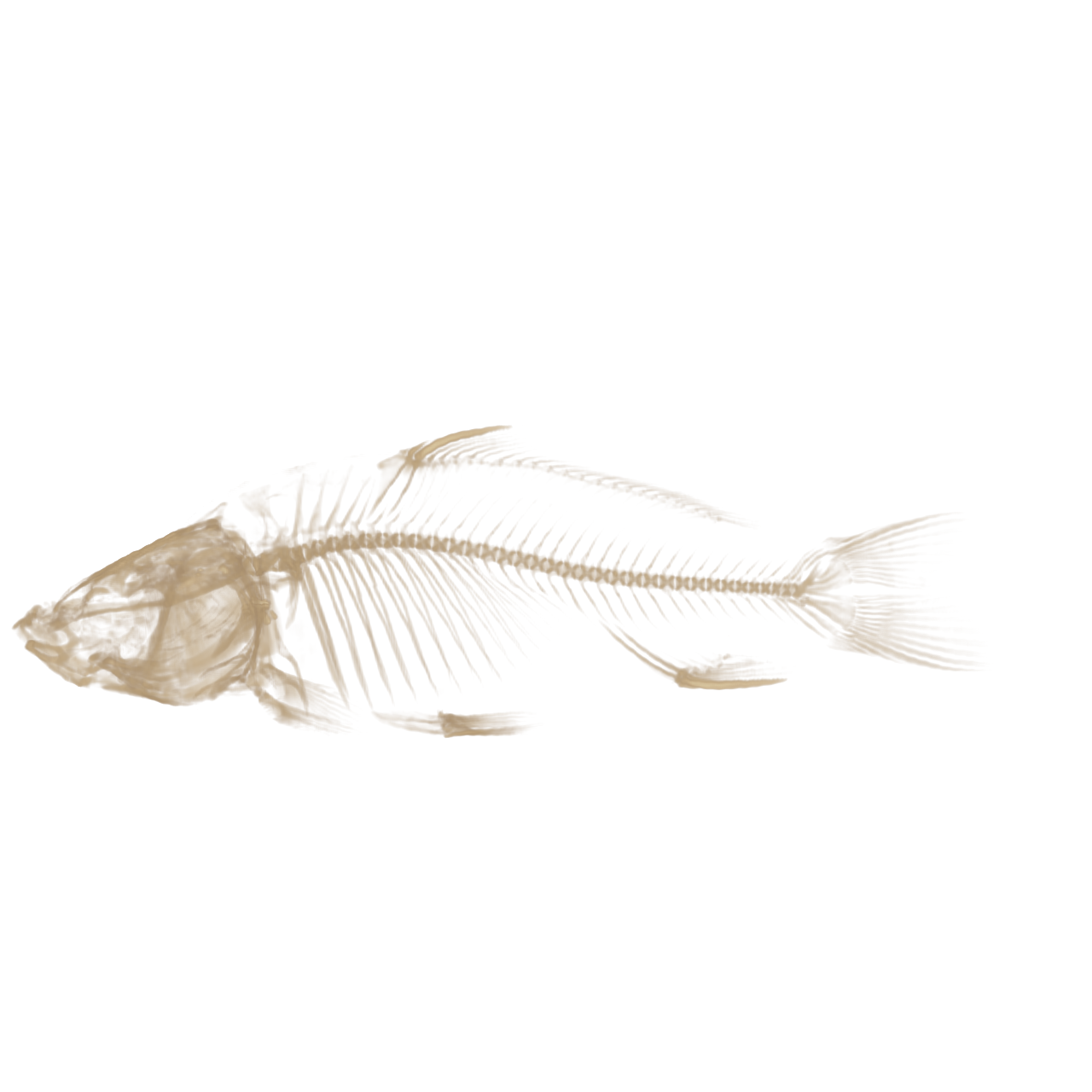
Task: Load the carp dataset from "carp/data/carp_256x256x512_uint16.raw", the information about this dataset: Carp (Scalar) Data Scalar Type: unsigned short Data Byte Order: little Endian Data Spacing: 0.78125x0.390625x1 Data Extent: 256x256x512 Instructions: 1. Load the dataset into ParaView. 2. Apply volume rendering to visualize the carp skeleton. 3. Adjust the transfer function to highlight only the bony structures with the original bone color. 4. Optimize the viewpoint to display the full skeleton, ensuring the head, spine, and fins are all clearly visible in a single frame. 5. Analyze the visualization and answer the following questions: Q1: Which of the following options correctly describes the fins visible in the carp skeleton visualization? A. 5 fins: 1 dorsal, 2 pectoral, 2 pelvic B. 6 fins: 1 dorsal, 2 pectoral, 2 pelvic, 1 caudal C. 7 fins: 1 dorsal, 2 pectoral, 2 pelvic, 1 anal, 1 caudal D. 8 fins: 2 dorsal, 2 pectoral, 2 pelvic, 1 anal, 1 caudal Q2: Based on the visualization, what is the approximate ratio of skull length to total body length? A. ~15% B. ~22% C. ~30% D. ~40% 6. Use a white background. Find an optimal view. Render at 1280x1280. Do not show a color bar or coordinate axes. 7. Set the viewpoint parameters as: [265.81, 1024.69, 131.23] to position; [141.24, 216.61, 243.16] to focal point; [0.99, -0.14, 0.07] to camera up direction. 8. Save your work: Save the visualization image as "carp/results/{agent_mode}/carp.png". Save the answers to the analysis questions in plain text as "carp/results/{agent_mode}/answers.txt". (Optional, but must save if use paraview) Save the paraview state as "carp/results/{agent_mode}/carp.pvsm". (Optional, but must save if use pvpython script) Save the python script as "carp/results/{agent_mode}/carp.py". (Optional, but must save if use VTK) Save the cxx code script as "carp/results/{agent_mode}/carp.cxx" Do not save any other files, and always save the visualization image and the text file.

🖼️ Visualization Comparison

Ground Truth

Agent Result

📏 Vision Evaluation Rubrics

Score Summary

Total Score

23/30

Goals

3

Points/Goal

10

Goal 1

8/10

Criterion: Overall Visualization Goal: Does the result match the ground truth visualization of the carp skeleton?

Judge's Assessment: The result image shows a full carp skeleton in a similar left-facing side view on a white background, matching the ground truth’s overall composition (head at left, tail at right, spine arcing slightly). However, the rendering/transfer function differs: the result is darker/browner overall and slightly more opaque in the skull region, while the ground truth is paler and more uniformly bone-colored. The viewpoint/framing is close but not identical in perceived scale and tonal balance.

Goal 2

7/10

Criterion: Bone Visibility: Are the bones clearly visible, similar to the ground truth? Are thin fin rays distinguishable?

Judge's Assessment: Major bony structures (skull, vertebrae, ribs) are clearly visible, and fin rays are present. Compared to the ground truth, some thin structures—especially in the dorsal and caudal fin rays—appear a bit more washed out/blurred in the result, reducing crispness and separability of individual rays. The skull region is also comparatively denser, which can obscure fine bone detail versus the ground truth’s lighter appearance.

Goal 3

8/10

Criterion: Skeletal Structure: Is the entire carp skeleton (head, spine, ribs, fins, tail) visible and similar in appearance to the ground truth?

Judge's Assessment: The complete skeletal anatomy is shown: skull, spine/vertebrae, rib cage, dorsal fin, paired fins, and caudal fin are all visible in one frame, consistent with the ground truth. Differences are mainly in contrast/opacity and bone color (result is darker and slightly hazier), but the overall structural completeness and similarity are good.

Overall Assessment

The result successfully visualizes the full carp skeleton with appropriate orientation and white background, closely matching the ground truth in structure and framing. The primary mismatches are transfer-function/opacity and color tone: the result is darker and slightly hazier, which reduces the crisp visibility of thin fin rays compared with the ground truth.

📝 Text-Based Q&A Evaluation

Score

10/20 (50.0%)

Questions & Correct Answers

Q1 correct answer: C. 7 fins: 1 dorsal, 2 pectoral, 2 pelvic, 1 anal, 1 caudal

Q2 correct answer: B. ~22%

Agent's Answers

Q1: Which of the following options correctly describes the fins visible in the carp skeleton visualization?
Answer: C. 7 fins: 1 dorsal, 2 pectoral, 2 pelvic, 1 anal, 1 caudal

Explanation: Based on the volume-rendered skeleton visualization, I can identify the following fins:
- 1 dorsal fin located on the top of the back
- 2 pectoral fins positioned near the head region on both sides
- 2 pelvic fins located in the ventral area on both sides
- 1 anal fin positioned on the bottom near the tail region
- 1 caudal fin at the tail end
This gives a total of 7 fins, which is typical for cyprinid fish like carp.

Q2: Based on the visualization, what is the approximate ratio of skull length to total body length?
Answer: A. ~15%

Explanation: By examining the skeleton visualization, the skull (cranium) extends from the anterior tip of the mouth to approximately the posterior edge of the gill structures where the pectoral fins attach. Comparing this length to the total body length (from the mouth tip to the end of the caudal fin), the skull length represents approximately 15% of the total body length.

Judge's Evaluation

Evaluation:

Criterion 1 (Q1, /10): 10/10. The answer selects option C and describes 7 fins with the correct breakdown (1 dorsal, 2 pectoral, 2 pelvic, 1 anal, 1 caudal), matching the stated correct answer exactly. Criterion 2 (Q2, /10): 0/10. The answer selects option A (~15%) and justifies it, but the evaluation criterion specifies the correct answer is B (~22%). Since the chosen option and numeric estimate do not match the required criterion, it does not meet the correctness requirement.

📊 Detailed Metrics

Visualization Quality

23/30

Output Generation

5/5

Efficiency

8/10

Completed in 127.94 seconds (good)

PSNR

33.85 dB

SSIM

0.9845

LPIPS

0.0176

Text Q&A Score

10/20

50.0%

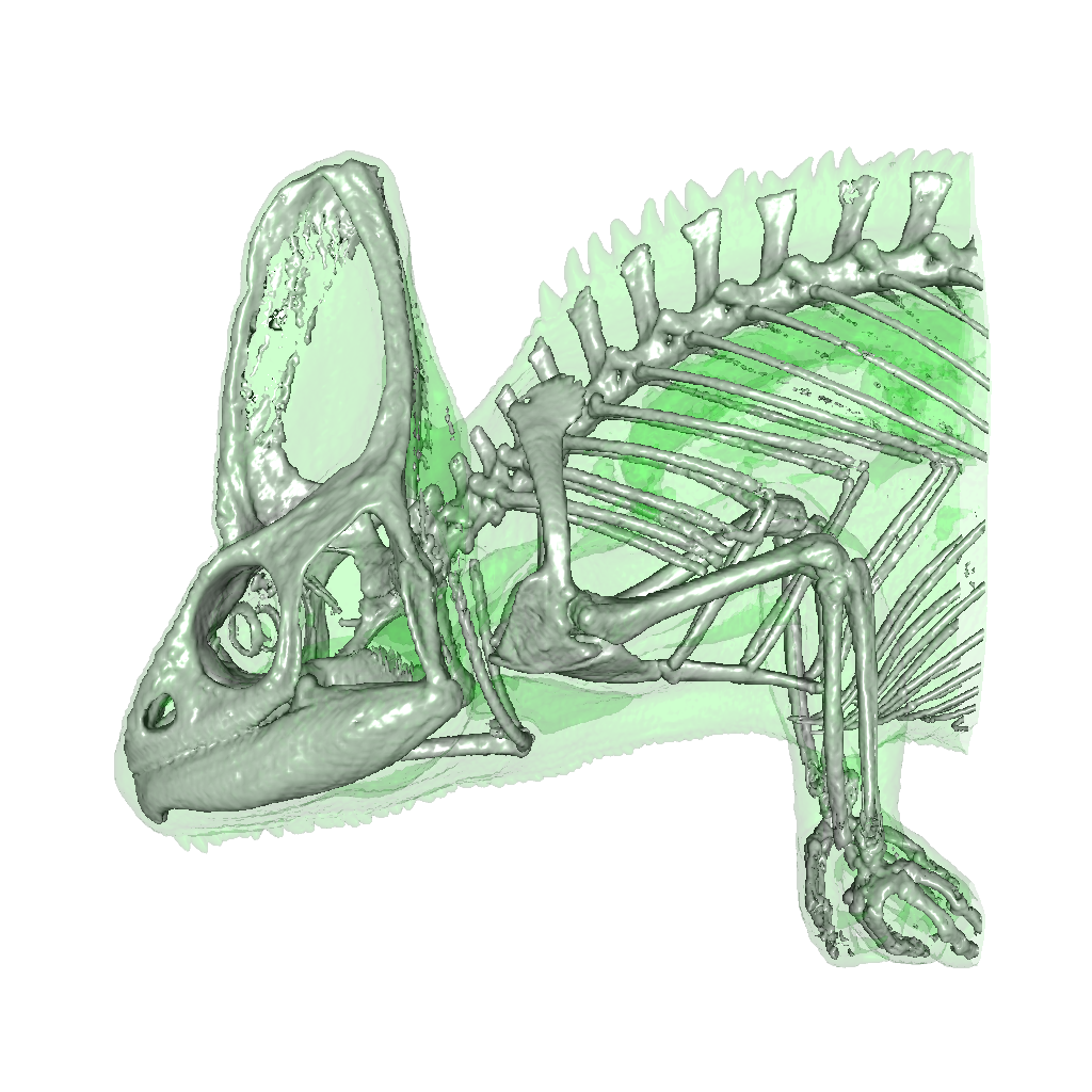
📝 chameleon_isosurface

36/45 (80.0%)

📋 Task Description

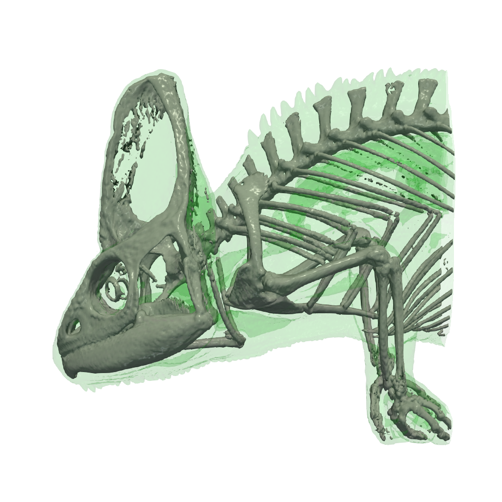
Task: Load the chameleon dataset from "chameleon_isosurface/data/chameleon_isosurface_256x256x256_float32.vtk". Generate a visualization image of 2 isosurfaces of the Chameleon scalar field dataset with the following visualization settings: 1) Create isosurfaces of Iso_1 with a value of 0.12 and Iso_2 with a value of 0.45 2) Assign RGB color of [0.0, 1.0, 0.0] to Iso_1, and color of [1.0, 1.0, 1.0] to Iso_2 3) Assign opacity of 0.1 to Iso_1, and opacity of 0.99 to Iso_2 4) Set the lighting parameter as: 0.1 to Ambient; 0.7 to Diffuse; 0.6 to Specular 5) Set the viewpoint parameters as: [600, 0, 0] to position; [0, 0, 0] to focal point; [0, -1, 0] to camera up direction 6) White background 7) Visualization image resolution is 1024x1024 8) Don't show color/scalar bar or coordinate axes. Save the visualization image as "chameleon_isosurface/results/{agent_mode}/chameleon_isosurface.png". (Optional, but must save if use paraview) Save the paraview state as "chameleon_isosurface/results/{agent_mode}/chameleon_isosurface.pvsm". (Optional, but must save if use pvpython script) Save the python script as "chameleon_isosurface/results/{agent_mode}/chameleon_isosurface.py". (Optional, but must save if use VTK) Save the cxx code script as "chameleon_isosurface/results/{agent_mode}/chameleon_isosurface.cxx" Do not save any other files, and always save the visualization image.

🖼️ Visualization Comparison

Ground Truth

Agent Result

📏 Vision Evaluation Rubrics

Score Summary

Total Score

23/30

Goals

3

Points/Goal

10

Goal 1

9/10

Criterion: Does the result present 2 isosurfaces, one showing the inner part of the chameleon and one showing the outer part of the chameleon?

Judge's Assessment: The result shows two distinct isosurfaces similar to the ground truth: a translucent outer shell/skin around the chameleon and a much more opaque inner skeletal/bony structure (skull, ribs, limbs, spine). The separation and overall morphology match very well, with only minor differences in shading/contrast compared to the ground truth.

Goal 2

8/10

Criterion: Is the skin of the Chameleon object of green color?

Judge's Assessment: The outer skin is clearly green and semi-transparent as in the ground truth. However, the green appears slightly darker/more saturated in places and the translucency/lighting balance differs a bit, making the skin read less uniformly pale-green than the reference.

Goal 3

6/10

Criterion: Is the bone of the Chameleon object of white color?

Judge's Assessment: The inner 'bone' structure is present and stands out, but in the result it appears more gray/greenish-gray than clean white as in the ground truth. The whiteness is reduced due to lighting/material appearance, so it does not match the reference bone color closely.

Overall Assessment

Overall geometry and the presence of both inner and outer isosurfaces match the ground truth well. The main discrepancy is material/color rendering: the skin is acceptably green, but the bones are noticeably less white (more gray), reducing fidelity to the intended coloring.

📊 Detailed Metrics

Visualization Quality

23/30

Output Generation

5/5

Efficiency

8/10

Completed in 152.44 seconds (good)

📝 chart-opacity

37/55 (67.3%)

📋 Task Description

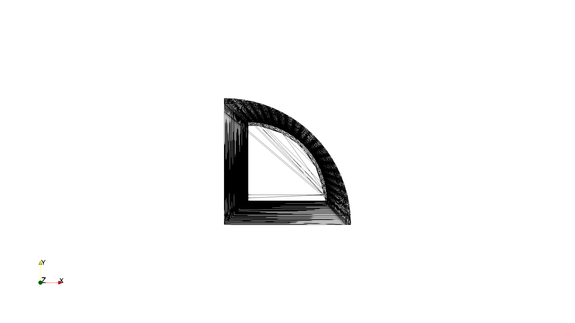
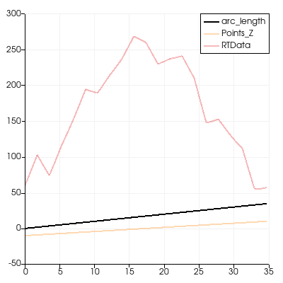
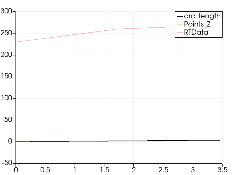
Create a wavelet object. Create a plot over line chart from the wavelet with three paths: arc_length, Points_Z, and RTData variables with opacity for arc_length 1 and opacity for Points_Z and RTData 0.3. Save the visualization image as "chart-opacity/results/{agent_mode}/chart-opacity.png". (Optional, but must save if use paraview) Save the paraview state as "chart-opacity/results/{agent_mode}/chart-opacity.pvsm". (Optional, but must save if use python script) Save the python script as "chart-opacity/results/{agent_mode}/chart-opacity.py". Do not save any other files, and always save the visualization image.

🖼️ Visualization Comparison

Ground Truth

Agent Result

📏 Vision Evaluation Rubrics

Score Summary

Total Score

22/40

Goals

4

Points/Goal

10

Goal 1

6/10

Criterion: Chart Generation: Is the plot over line chart properly created from the wavelet data?

Judge's Assessment: Both ground truth and result show a line-chart style plot with three series and a legend, consistent with a Plot Over Line output. However, the result’s x-axis range/scale (0–3.5) differs markedly from the ground truth (0–35), and the overall curve shapes suggest the plotted sampling/domain is not matching the expected plot-over-line output from the wavelet.

Goal 2

7/10

Criterion: Variable Display: Are arc_length, Points_Z, and RTData variables all correctly plotted, showing all three specified variables and distinguishable in the chart?

Judge's Assessment: The result includes all three variables (arc_length in black, Points_Z in orange, RTData in pink/red) and they are distinguishable via color and legend entries. Nonetheless, the data trends do not match the ground truth: in the ground truth RTData has a strong peak and then declines, while in the result RTData is nearly monotonic and much smoother; arc_length and Points_Z also appear flatter/compressed compared to the ground truth.

Goal 3

3/10

Criterion: Opacity Settings: Is the arc_length variable displayed with full opacity (1.0) while Points_Z and RTData show reduced opacity (0.3)?

Judge's Assessment: Opacity does not appear to match the requirement/ground truth. In the ground truth, Points_Z and RTData look clearly lighter (semi-transparent) than arc_length. In the result, the RTData and Points_Z lines appear close to fully opaque (similar visual weight/opacity to a normal line), so the intended 0.3 opacity effect is not convincingly present.

Goal 4

6/10

Criterion: Chart Clarity: Does the chart provide clear visualization of the data trends with appropriate axis scaling and readable formatting?

Judge's Assessment: The chart is readable with gridlines and a clear legend, but axis scaling differs from the ground truth (notably x-axis extent), which changes how trends are perceived and compresses the lower-valued series near zero. Overall clarity is acceptable, but it does not match the expected formatting/scaling and makes comparison between series less informative than in the ground truth.

Overall Assessment

The result produces a readable multi-series line chart with the correct variable names, but it does not match the ground truth’s domain/trends and fails to clearly apply the required opacity differences (arc_length opaque; Points_Z and RTData semi-transparent). The main mismatches are the x-axis range/data behavior and the missing/insufficient transparency effect.

📊 Detailed Metrics

Visualization Quality

22/40

Output Generation

5/5

Efficiency

10/10

Completed in 43.74 seconds (excellent)

📝 climate

31/45 (68.9%)

📋 Task Description

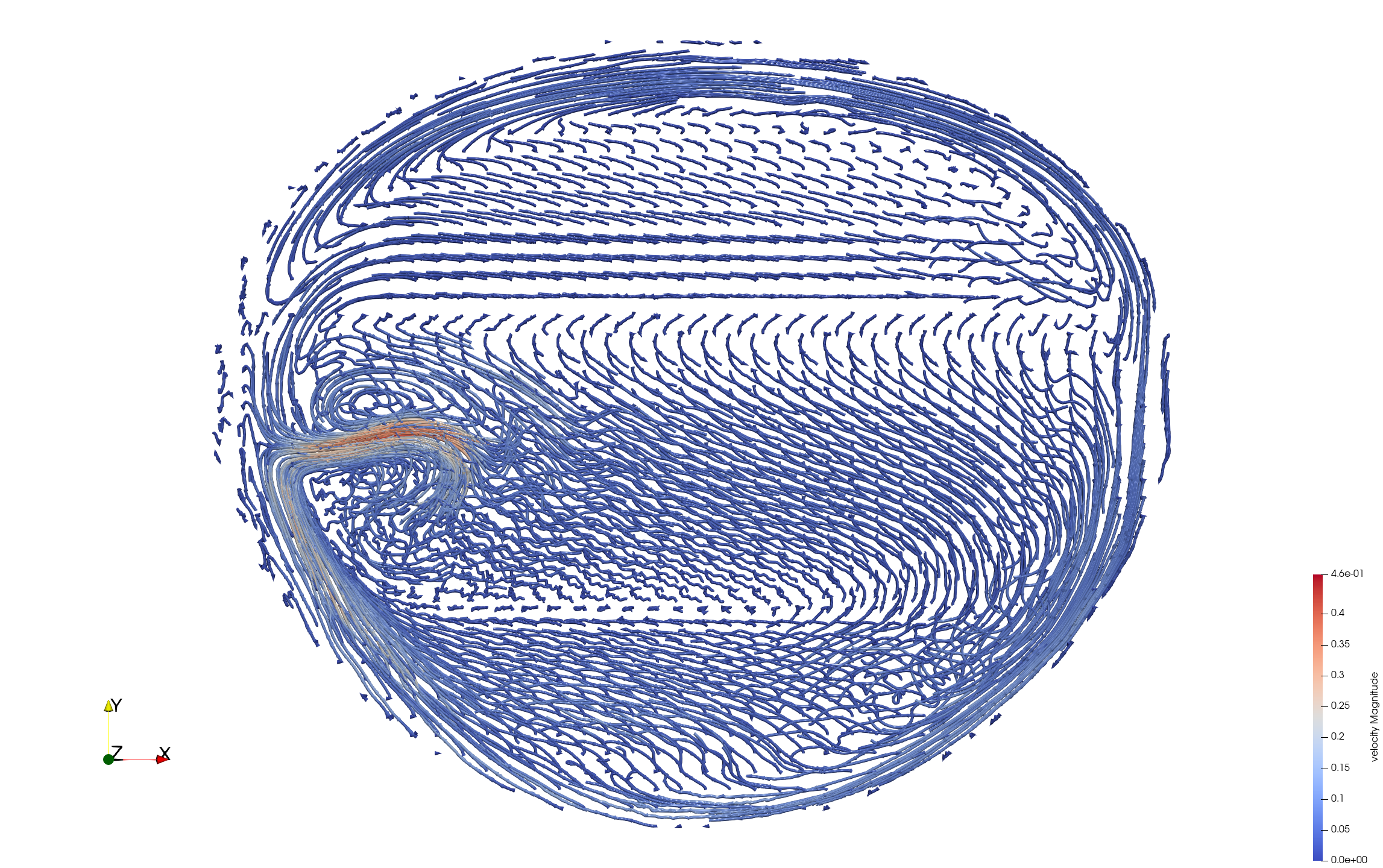
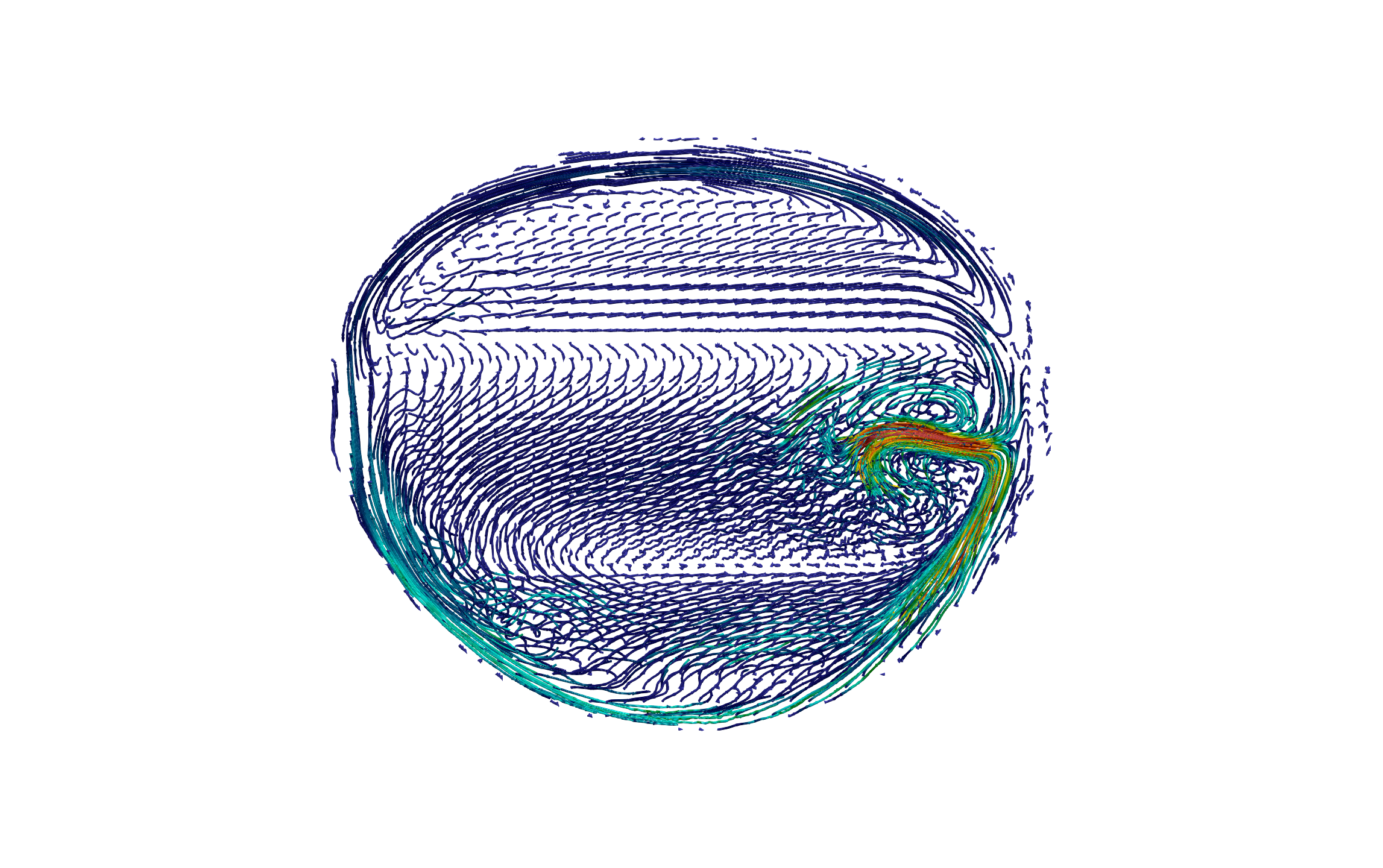
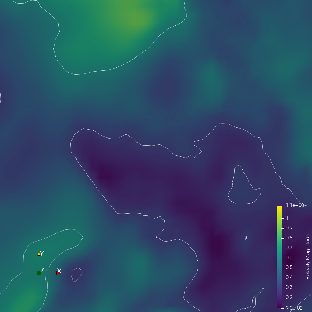
I would like to use ParaView to visualize a dataset of ocean currents. Read in the file named "climate/data/climate.vtp". Apply a calculator filter to compute the following function: (-velocity_X*sin(coordsX*0.0174533) + velocity_Y*cos(coordsX*0.0174533)) * iHat + (-velocity_X * sin(coordsY*0.0174533) * cos(coordsX*0.0174533) - velocity_Y * sin(coordsY*0.0174533) * sin(coordsX*0.0174533) + velocity_Z * cos(coordsY*0.0174533)) * jHat + 0*kHat Render the computed values using a tube filter with 0.05 as the tube radius. Color the tubes by the magnitude of the velocity. Light the tubes with the maximum shininess and include normals in the lighting. Add cone glyphs to show the direction of the velocity. The glyphs are composed of 10 polygons, having a radius 0 0.15, a height of 0.5, and a scaling factor of 0.5. View the result in the -z direction. Adjust the view so that the tubes occupy the 90% of the image. Save a screenshot of the result, 2294 x 1440 pixels, white background, in the filename "climate/results/{agent_mode}/climate.png". (Optional, but must save if use paraview) Save the paraview state as "climate/results/{agent_mode}/climate.pvsm". (Optional, but must save if use python script) Save the python script as "climate/results/{agent_mode}/climate.py". Do not save any other files, and always save the visualization image.

🖼️ Visualization Comparison

Ground Truth

Agent Result

📏 Vision Evaluation Rubrics

Score Summary

Total Score

18/30

Goals

3

Points/Goal

10

Goal 1

7/10

Criterion: Tube Visualization: Are the tubes rendered with correct radius (0.05), colored by velocity magnitude, and proper lighting with maximum shininess?

Judge's Assessment: Ground truth shows tubes colored by velocity magnitude with a mostly dark-blue field and a localized higher-magnitude region (orange/red) on the left; lighting looks glossy and the tube thickness appears uniform. The result image also uses tubes and a magnitude colormap, but the high-magnitude region appears on the right and the overall color distribution differs (more green/cyan around the lower rim). This indicates either different computed vectors (calculator) and/or different scalar range mapping. Tube radius/shading look broadly similar, but not a close match to the ground truth.

Goal 2

6/10

Criterion: Cone Glyph Direction: Are the cone glyphs properly configured with specified parameters and showing velocity direction accurately?

Judge's Assessment: Both images include dense cone/arrow-like glyphs indicating direction along the flow lines. However, the direction field pattern is not matching the ground truth (notably the main energetic jet/feature is on the opposite side), and the glyph prominence/spacing appears somewhat different. While cones are present and generally aligned with the flow, the mismatch suggests the glyphs are not showing the same computed velocity direction as the ground truth.

Goal 3

5/10

Criterion: View Configuration: Is the visualization displayed from -z direction with appropriate scaling and white background as specified?

Judge's Assessment: Both views are on a white background and appear to be from the -Z direction (top-down). However, the framing/zoom differs: ground truth fills most of the image (~90%) and includes a colorbar and axis triad, while the result is more zoomed out with much more whitespace and no visible scalar bar/triad. The overall orientation also appears horizontally mirrored (main feature left vs right).

Overall Assessment

The result captures the general visualization elements (tubes colored by magnitude and cone glyphs on a white background, viewed roughly top-down), but it does not match the ground truth in key visual aspects: the main high-velocity feature is on the opposite side, the magnitude color distribution differs, and the view framing is not scaled to fill ~90% of the image. These differences suggest an inconsistency in the calculator transform and/or camera setup compared to the reference.

📊 Detailed Metrics

Visualization Quality

18/30

Output Generation

5/5

Efficiency

8/10

Completed in 144.52 seconds (good)

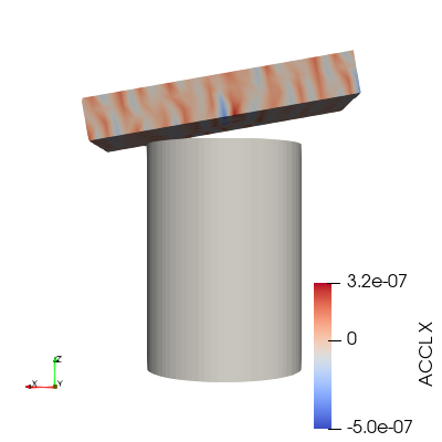
📝 color-blocks

49/55 (89.1%)

📋 Task Description

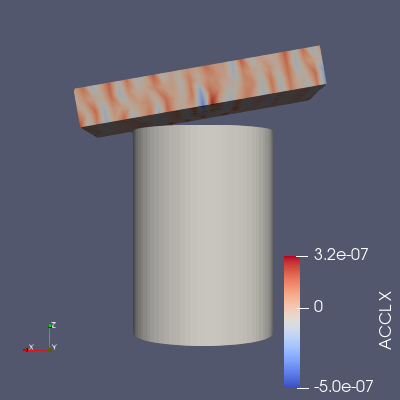
I would like to use ParaView to visualize a dataset. Set the background to a blue-gray palette. Read the file "color-blocks/data/color-blocks.ex2". This is a multiblock dataset. Color the dataset by the vtkBlockColors field. Retrieve the color map for vtkBlockColors. Retrieve the opacity transfer function for vtkBlockColors. Retrieve the 2D transfer function for vtkBlockColors. Set block coloring for the block at /IOSS/element_blocks/block_2 using the variable ACCL on the x component of the points. Rescale the block's color and opacity maps to match the current data range of block_2. Retrieve the color transfer function for the ACCL variable of block_2. Enable the color bar for block_2. Apply a cool to warm color preset to the color map for block_2. Set the camera to look down the -y direction and to see the entire dataset. Save the visualization image as "color-blocks/results/{agent_mode}/color-blocks.png". (Optional, but must save if use paraview) Save the paraview state as "color-blocks/results/{agent_mode}/color-blocks.pvsm". (Optional, but must save if use python script) Save the python script as "color-blocks/results/{agent_mode}/color-blocks.py". Do not save any other files, and always save the visualization image.

🖼️ Visualization Comparison

Ground Truth

Agent Result

📏 Vision Evaluation Rubrics

Score Summary

Total Score

36/40

Goals

4

Points/Goal

10

Goal 1

7/10

Criterion: Block Color Mapping: Is the dataset properly colored by vtkBlockColors field with distinct block visualization?

Judge's Assessment: In the ground truth, the multiblock structure is evident: the cylinder and the top beam are distinct blocks, with the beam showing the ACCL-based coloring while the cylinder remains a uniform neutral color. In the result, the same two main blocks are visible and similarly separated. However, the expected explicit vtkBlockColors-based distinct block coloring is not clearly demonstrated beyond the neutral cylinder vs. colored beam, so it only partially confirms correct vtkBlockColors usage.

Goal 2

9/10

Criterion: Individual Block Coloring: Is block_2 correctly colored using the x component of the ACCL variable with appropriate scaling?

Judge's Assessment: The top block (corresponding to block_2) in the result is colored with a smooth cool-to-warm diverging pattern consistent with an ACCL X-component field, while the cylinder remains uncolored/solid. The data range on the color bar matches the ground truth (about -5.0e-07 to 3.2e-07 with 0 centered), indicating the rescale to current data range is correctly applied. Minor differences in shading/contrast are negligible.

Goal 3

10/10

Criterion: Color Transfer Functions: Are the color transfer functions properly applied with cool to warm coloring for the ACCL variable?

Judge's Assessment: The result uses the same cool-to-warm diverging transfer function as the ground truth for ACCL X (blue negative, red positive, white near zero) with the same tick labeling and range appearance, matching extremely closely.

Goal 4

10/10

Criterion: View Configuration: Is the dataset displayed from the -y direction with blue-gray background and visible color bar legend?

Judge's Assessment: The result matches the ground truth view configuration: camera looks from the -y direction with the full dataset in view, the background is the intended blue-gray palette, and the vertical color bar legend labeled "ACCL X" is visible on the right.

Overall Assessment

The result is an excellent match overall: the ACCL X coloring on block_2, the cool-to-warm transfer function, the color bar, background, and camera orientation all closely match the ground truth. The only notable uncertainty is whether vtkBlockColors-based block coloring is explicitly and fully reflected beyond the obvious separation of the two main blocks.

📊 Detailed Metrics

Visualization Quality

36/40

Output Generation

5/5

Efficiency

8/10

Completed in 142.25 seconds (good)

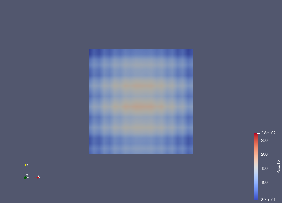
📝 color-data

44/45 (97.8%)

📋 Task Description

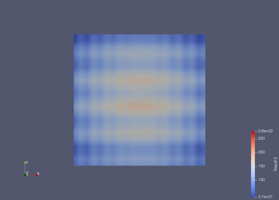
Create a wavelet object. Create a new calculator with the function 'RTData*iHat + ln(RTData)*jHat + coordsZ*kHat'. Get a color transfer function/color map and opacity transfer function/opacity map for the result of the calculation, scaling the color and/or opacity maps to the data range. For a surface representation, color by the x coordinate of the result using a cool to warm color map, show the color bar/color legend, and save a screenshot of size 1158 x 833 pixels in "color-data/results/{agent_mode}/color-data.png". (Optional, but must save if use paraview) Save the paraview state as "color-data/results/{agent_mode}/color-data.pvsm". (Optional, but must save if use python script) Save the python script as "color-data/results/{agent_mode}/color-data.py". Do not save any other files, and always save the visualization image.

🖼️ Visualization Comparison

Ground Truth

Agent Result

📏 Vision Evaluation Rubrics

Score Summary

Total Score

29/30

Goals

3

Points/Goal

10

Goal 1

10/10

Criterion: Color Transfer Function: Is the color transfer function correctly applied with cool to warm color mapping scaled to the data range?

Judge's Assessment: The result uses the same cool-to-warm (blue→white→red) transfer function as the ground truth, with matching overall hues and a similar distribution of blues at the edges and warmer tones in the interior. The color bar range also matches (approximately 3.7e+01 to 2.8e+02), indicating the map is scaled to the data range similarly to the ground truth.

Goal 2

9/10

Criterion: Surface Coloring: Is the surface representation properly colored by the x coordinate of the calculated result?

Judge's Assessment: The surface is colored by the calculated result’s X component (label shown as “Result X”), matching the ground truth field selection and producing the same banded/striped pattern across the plane. Minor differences in framing/zoom (object appears slightly larger in the result) do not materially affect the correctness of the surface coloring.

Goal 3

10/10

Criterion: Color Bar Display: Is the color bar/legend visible and properly displaying the color mapping scale and values?

Judge's Assessment: A vertical color bar/legend is visible on the right in the result, labeled “Result X”, with tick marks and numeric values matching the ground truth styling and range. Placement and readability are consistent with the expected output.

Overall Assessment

The generated visualization matches the ground truth very closely: correct cool-to-warm color mapping scaled to the data range, correct coloring by Result X on a surface, and a properly displayed color legend. Only a slight difference in zoom/framing is noticeable.

📊 Detailed Metrics

Visualization Quality

29/30

Output Generation

5/5

Efficiency

10/10

Completed in 57.52 seconds (excellent)

📝 crayfish_streamline

31/45 (68.9%)

📋 Task Description

Load the Crayfish flow vector field from "crayfish_streamline/data/crayfish_streamline_322x162x119_float32_scalar3.raw", the information about this dataset: Crayfish Flow (Vector) Data Scalar Type: float Data Byte Order: Little Endian Data Extent: 322x162x119 Number of Scalar Components: 3 Data loading is very important, make sure you correctly load the dataset according to their features. Create two streamline sets using "Stream Tracer" filters with "Point Cloud" seed type, each with 100 seed points and radius 32.2: - Streamline 1: Seed center at [107.33, 81.0, 59.5]. Apply a "Tube" filter (radius 0.5, 12 sides). Color by Velocity magnitude using a diverging colormap with the following RGB control points: - Value 0.0 -> RGB(0.231, 0.298, 0.753) (blue) - Value 0.02 -> RGB(0.865, 0.865, 0.865) (white) - Value 0.15 -> RGB(0.706, 0.016, 0.149) (red) - Streamline 2: Seed center at [214.67, 81.0, 59.5]. Apply a "Tube" filter (radius 0.5, 12 sides). Color by Velocity magnitude using the same colormap. Show the dataset bounding box as an outline (black). In the pipeline browser panel, hide all stream tracers and only show the tube filters and the outline. Use a white background. Render at 1280x1280. Set the viewpoint parameters as: [436.67, -370.55, 562.71] to position; [160.5, 80.5, 59.07] to focal point; [-0.099, 0.714, 0.693] to camera up direction Save the paraview state as "crayfish_streamline/results/{agent_mode}/crayfish_streamline.pvsm". Save the visualization image as "crayfish_streamline/results/{agent_mode}/crayfish_streamline.png". (Optional, if use python script) Save the python script as "crayfish_streamline/results/{agent_mode}/crayfish_streamline.py". Do not save any other files, and always save the visualization image.

🖼️ Visualization Comparison

Ground Truth

Agent Result

📏 Vision Evaluation Rubrics

Score Summary

Total Score

18/30

Goals

3

Points/Goal

10

Goal 1

6/10

Criterion: Overall Visualization Goal: Does the result show streamline tubes colored by velocity magnitude within a rectangular bounding box, similar to the ground truth?

Judge's Assessment: Ground truth shows two dense streamline tube bundles inside a black outline bounding box on a white background with the specified oblique camera view and a visible scalar bar. The result also shows two streamline-like tube bundles inside an outline box, but the presentation differs notably: background is dark gray (not white), camera/view is different (more head-on/orthographic-looking), and the overall styling/lighting makes the scene look substantially different from the ground truth even though the core objects are present.

Goal 2

8/10

Criterion: Streamline Clusters: Are there two distinct clusters that matches the ground truth layout?

Judge's Assessment: Both images clearly contain two distinct streamline clusters (left and right) in approximately the same overall spatial arrangement inside the box. The relative separation and the notion of two seed regions are preserved. Minor differences exist in apparent spread and density/extent of the lines, likely due to different integration/seeding/display settings or camera.

Goal 3

4/10

Criterion: Color Mapping: Are the tubes colored by velocity magnitude using a blue-white-red diverging colormap, with a similar distribution as the ground truth?

Judge's Assessment: Ground truth uses a blue-white-red diverging map with a strong presence of blues on many outer streamlines and reds/whites intermingled, matching a vorticity-magnitude diverging scheme. The result image is dominated by reds and grays with little to no blue visible, which does not match the expected diverging blue-white-red appearance or distribution; it suggests a different colormap, different scalar range, or different quantity being colored.

Overall Assessment

The result captures the key geometric requirement of two streamline tube clusters within a bounding box, but it diverges substantially in rendering setup (background and camera) and especially in color mapping, where the expected blue-white-red diverging appearance is not reproduced.

📊 Detailed Metrics

Visualization Quality

18/30

Output Generation

5/5

Efficiency

8/10

Completed in 97.88 seconds (good)

PSNR

19.91 dB

SSIM

0.9306

LPIPS

0.0794

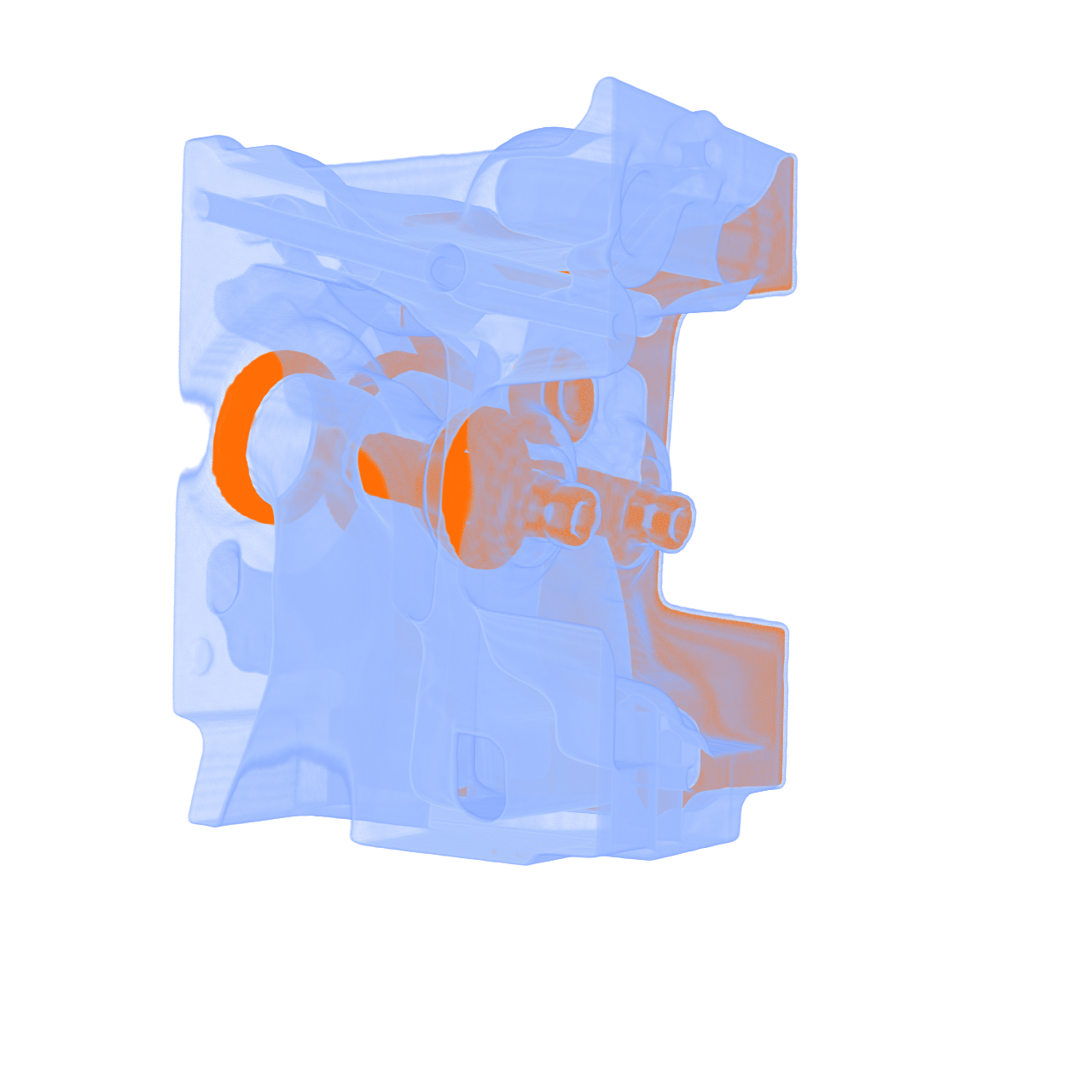
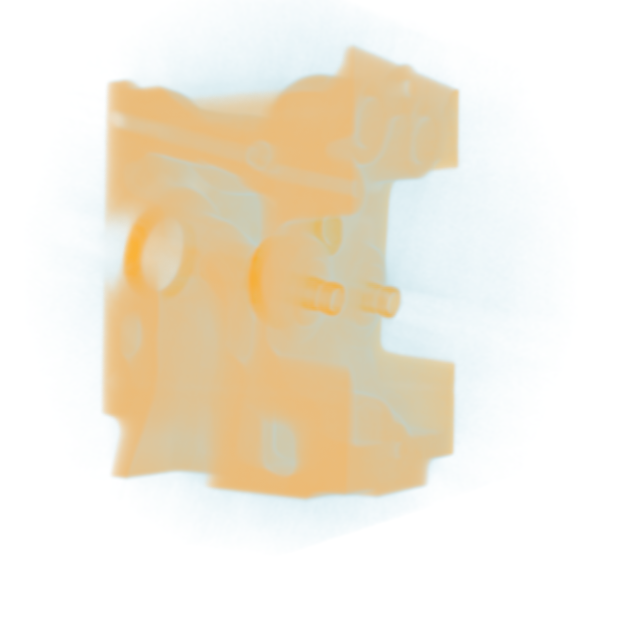
📝 engine

⚠️ LOW SCORE

26/55 (47.3%)

📋 Task Description

Task: Load the vortex dataset from "engine/data/engine_256x256x128_uint8.raw", the information about this dataset: engine (Scalar) Data Scalar Type: float Data Byte Order: little Endian Data Extent: 256x256x128 Number of Scalar Components: 1 Instructions: 1. Load the dataset into ParaView. 2. Apply the volume rendering to visualize the engine dataset 3. Adjust the transfer function, let the outer part more transparent and the inner part more solid. Use light blue for the outer part and orange for the inner part. 4. Use a white background. Find an optimal view. Render at 1280x1280. Do not show a color bar or coordinate axes. 5. Set the viewpoint parameters as: [-184.58, 109.48, -431.72] to position; [134.05, 105.62, 88.92] to focal point; [0.01, 1.0, -0.001] to camera up direction. 6. Save your work: Save the visualization image as "engine/results/{agent_mode}/engine.png". (Optional, but must save if use paraview) Save the paraview state as "engine/results/{agent_mode}/engine.pvsm". (Optional, but must save if use pvpython script) Save the python script as "engine/results/{agent_mode}/engine.py". (Optional, but must save if use VTK) Save the cxx code script as "engine/results/{agent_mode}/engine.cxx" Do not save any other files, and always save the visualization image.

🖼️ Visualization Comparison

Ground Truth

Agent Result

📏 Vision Evaluation Rubrics

Score Summary

Total Score

13/40

Goals

4

Points/Goal

10

Goal 1

4/10

Criterion: Overall Visualization Goal: How well does the result use volume rendering to clearly present the internal and external structures of the engine dataset?

Judge's Assessment: Ground truth shows a crisp volume rendering with a clearly visible engine block: translucent light-blue exterior and distinct orange internal parts (cylindrical cavities/shafts) with sharp boundaries. The result image looks heavily over-smoothed/over-exposed (very hazy), with much weaker structural definition; the overall engine shape is present but internal/external features are not clearly conveyed via volume rendering.

Goal 2

3/10

Criterion: Structural Clarity: Does the visualization emphasize depth so that the outer layers do not obscure the inner structures?

Judge's Assessment: In the ground truth, depth layering is strong: the outer shell is transparent enough to reveal internal orange structures without being washed out. In the result, the volume appears uniformly foggy and low-contrast, so depth cues are weak and internal details are difficult to discern; the outer layer does not provide a clear see-through shell effect.

Goal 3

2/10

Criterion: Transfer Function Transparency: Is the outer region rendered with higher transparency and the inner region more solid, achieving a clear layering effect?

Judge's Assessment: Ground truth achieves the requested transparency behavior: outer region is highly transparent while inner structures are more solid/opaque. The result looks almost uniformly semi-transparent with little separation between outer and inner opacity; the inner parts are not rendered with noticeably higher solidity than the exterior.

Goal 4

4/10

Criterion: Transfer Function Color Mapping: Are colors correctly assigned so that the outer part is light blue and the inner part is orange, enhancing structural contrast?

Judge's Assessment: Ground truth uses light blue for the exterior and saturated orange for the interior, creating strong contrast. The result is dominated by pale orange/beige with only faint hints of blue/teal; the intended blue exterior vs orange interior mapping is not clearly expressed.

Overall Assessment

Compared to the ground truth, the result captures the rough engine silhouette but fails to match the key visual goals: it is too washed-out and low-contrast, with poor depth separation and an incorrect/weak blue-vs-orange transfer function appearance. The outer/inner transparency layering that makes the ground truth effective is largely missing.

📊 Detailed Metrics

Visualization Quality

13/40

Output Generation

5/5

Efficiency

8/10

Completed in 103.59 seconds (good)

PSNR

22.78 dB

SSIM

0.9501

LPIPS

0.0913

📝 export-gltf

50/55 (90.9%)

📋 Task Description

Create a wavelet object. Create a surface rendering of the wavelet object and color by RTData. Scale the color map to the data, and don't display the color bar or the orientation axes. Export the view to "export-gltf/results/{agent_mode}/ExportedGLTF.gltf". Next load the file "export-gltf/results/{agent_mode}/ExportedGLTF.gltf" and display it as a surface. Color this object by TEXCOORD_0. Scale the color map to the data, and don't display the color bar or the orientation axes. Use the 'Cool to Warm' colormap. Set the background color to white. Save the visualization image as "export-gltf/results/{agent_mode}/export-gltf.png". (Optional, but must save if use paraview) Save the paraview state as "export-gltf/results/{agent_mode}/export-gltf.pvsm". (Optional, but must save if use python script) Save the python script as "export-gltf/results/{agent_mode}/export-gltf.py". Do not save any other files, and always save the visualization image.

🖼️ Visualization Comparison

Ground Truth

Agent Result

📏 Vision Evaluation Rubrics

Score Summary

Total Score

37/40

Goals

4

Points/Goal

10

Goal 1

9/10

Criterion: GLTF Export Quality: Is the wavelet object properly exported to GLTF format with correct surface representation and RTData coloring?

Judge's Assessment: The result shows the expected wavelet surface appearance with the characteristic banded cool-to-warm pattern (blue borders and reddish central bands), consistent with a successful export of the wavelet surface (originally colored by RTData) into GLTF. Any mismatch is minor and not clearly distinguishable from the images alone.

Goal 2

10/10

Criterion: GLTF Import and Display: Is the exported GLTF file successfully loaded and displayed as a surface with proper geometry?

Judge's Assessment: The imported GLTF is clearly displayed as a single square surface with the same overall geometry as the ground truth (flat, centered, square patch). No missing geometry or rendering artifacts are apparent.

Goal 3

8/10

Criterion: Texture Coordinate Coloring: Is the imported GLTF object correctly colored by TEXCOORD_0 with Cool to Warm colormap?

Judge's Assessment: The object is colored with a cool-to-warm scheme and the spatial pattern matches the ground truth well (horizontal red bands and bluish edges), indicating TEXCOORD_0-based coloring is likely applied. However, the result appears slightly different in framing/scale and perceived smoothness (the surface occupies more of the frame and looks a bit more blurred), suggesting minor differences in mapping/interpolation or camera setup.

Goal 4

10/10

Criterion: Clean Presentation: Are the color bar and orientation axes properly hidden for a clean visualization appearance?

Judge's Assessment: Both color bar and orientation axes are absent in the result, matching the clean presentation requirement. The background is white as specified.

Overall Assessment

The result closely matches the ground truth: correct surface geometry, clean view, and appropriate cool-to-warm coloring consistent with TEXCOORD_0. Minor differences are limited to framing and slight visual smoothness/blur, but core requirements are met.

📊 Detailed Metrics

Visualization Quality

37/40

Output Generation

5/5

Efficiency

8/10

Completed in 125.31 seconds (good)

📝 foot

33/45 (73.3%)

📋 Task Description

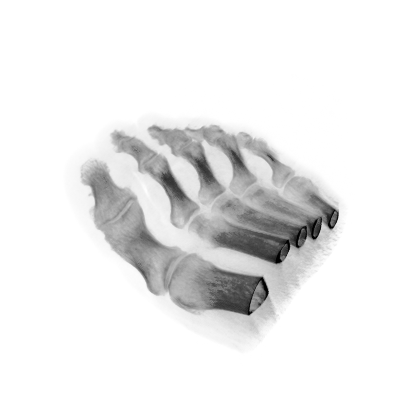
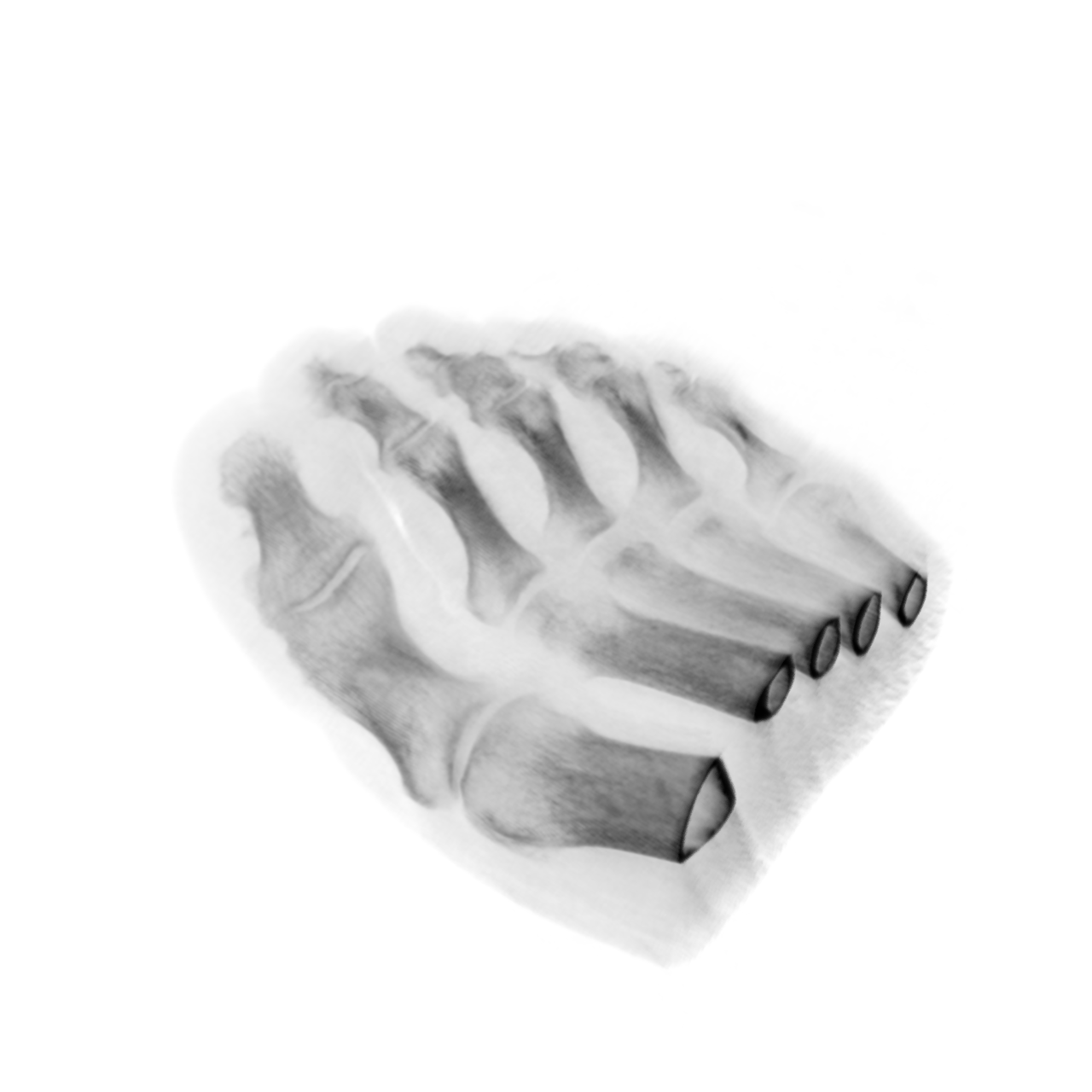
Task: Load the Foot dataset from "foot/data/foot_256x256x256_uint8.raw", the information about this dataset: Foot Description: Rotational C-arm x-ray scan of a human foot. Tissue and bone are present in the dataset. Data Type: uint8 Data Byte Order: little Endian Data Spacing: 1x1x1 Data Extent: 256x256x256 Data loading is very important, make sure you correctly load the dataset according to their features. Visualize the anatomical structures: 1. Apply volume rendering with an X-ray transfer function that distinguishes soft tissues and bones. Bones with darker color, and soft tissue with lighter color. 2. Analyze the visualization and answer the following questions: Q1: Based on the X-ray style volume rendering of the foot dataset, which of the following best describes the visibility of bony structures? A. Both the phalanges and metatarsals are fully visible B. The phalanges are fully visible, but the metatarsals are only partially visible C. The metatarsals are fully visible, but the phalanges are only partially visible D. Neither the phalanges nor the metatarsals are clearly visible 3. Use a white background. Find an optimal view. Render at 1280x1280. Do not show a color bar or coordinate axes. 4. Set the viewpoint parameters as: [-576.41, -264.41, -153.48] to position; [127.5, 127.5, 127.5] to focal point; [-0.52, 0.38, 0.76] to camera up direction. 5. Save your work: Save the visualization image as "foot/results/{agent_mode}/foot.png". Save the answers to the analysis questions in plain text as "foot/results/{agent_mode}/answers.txt". (Optional, but must save if use paraview) Save the paraview state as "foot/results/{agent_mode}/foot.pvsm". (Optional, but must save if use pvpython script) Save the python script as "foot/results/{agent_mode}/foot.py". (Optional, but must save if use VTK) Save the cxx code script as "foot/results/{agent_mode}/foot.cxx" Do not save any other files, and always save the visualization image and the text file.

🖼️ Visualization Comparison

Ground Truth

Agent Result

📏 Vision Evaluation Rubrics

Score Summary

Total Score

18/20

Goals

2

Points/Goal

10

Goal 1

9/10

Criterion: Overall Goal: Does the visualization effectively distinguish between different tissue types in the foot dataset?

Judge's Assessment: The result image matches the ground truth well in separating bony anatomy from surrounding soft tissue: bones appear as darker, higher-contrast structures while soft tissue is rendered lighter and more diffuse. The overall bone silhouettes (phalanges and metatarsals) are clearly visible with similar relative opacity to the ground truth. Minor differences exist in contrast/opacity—some regions in the result look slightly more washed out, reducing fine internal bone texture compared to the ground truth.

Goal 2

9/10

Criterion: X-ray Appearance: Does the visualization resemble an X-ray (monochrome or grayscale, transparent look, consistent lighting)?

Judge's Assessment: The rendering strongly resembles an X-ray style: grayscale, translucent volume appearance on a white background with smooth, consistent shading. The result is very close to the ground truth in tone mapping and transparency. Small deviations include slightly softer edges and marginally lower contrast in darker bony regions, but the overall X-ray aesthetic is preserved.

Overall Assessment

Overall, the agent-generated visualization is an excellent match to the ground truth: correct X-ray-like grayscale volume rendering on white background with clear visibility of major bony structures. Minor contrast/opacity differences slightly reduce crispness and internal detail compared to the reference, but the key goals are achieved.

📝 Text-Based Q&A Evaluation

Score

2/10 (20.0%)

Questions & Correct Answers

1. Q1 correct answer: B. The phalanges are fully visible, but the metatarsals are only partially visible

Agent's Answers

Q1: Based on the X-ray style volume rendering of the foot dataset, which of the following best describes the visibility of bony structures?

Answer: A. Both the phalanges and metatarsals are fully visible

Explanation: In the X-ray style volume rendering with darker colors for bones and lighter colors for soft tissue, both the phalanges (toe bones) and metatarsals (long bones of the foot) are clearly visible. The five phalanges at the front of the foot show distinct individual bones in dark color, and all five metatarsal bones connecting the toes to the midfoot are also fully visible with clear dark bone structures against the lighter soft tissue background.

Judge's Evaluation

Evaluation:

Criterion: Q1 correct answer is B (phalanges fully visible; metatarsals only partially visible). The provided answer selects A and explicitly claims both phalanges and metatarsals are fully visible. This directly contradicts the criterion regarding metatarsal visibility (they should be only partially visible). The explanation reinforces the incorrect choice by asserting all five metatarsals are fully visible with clear bone structures. Partial credit is warranted only insofar as the answer correctly states that the phalanges are fully visible, which aligns with the criterion. However, the key discriminating detail (metatarsals partially visible) is missed and replaced with the opposite claim, so the response largely fails to meet the evaluation criterion.

📊 Detailed Metrics

Visualization Quality

18/20

Output Generation

5/5

Efficiency

8/10

Completed in 95.36 seconds (good)

PSNR

30.33 dB

SSIM

0.9876

LPIPS

0.0382

Text Q&A Score

2/10

20.0%

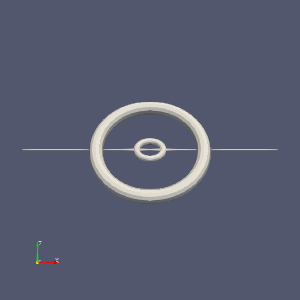
📝 import-gltf

46/55 (83.6%)

📋 Task Description

Load the "BlueGrayBackground" palette. Read the file "import-gltf/data/import-gltf.glb" and import the nodes "/assembly/Axle", "assembly/OuterRing/Torus002", and "assembly/OuterRing/MiddleRing/InnerRing". Set the layout size to 300x300 pixels. Point the camera in the positive Y direction and zoom to fit. Make sure all views are rendered, then save a screenshot to "import-gltf/results/{agent_mode}/import-gltf.png". (Optional, but must save if use paraview) Save the paraview state as "import-gltf/results/{agent_mode}/import-gltf.pvsm". (Optional, but must save if use python script) Save the python script as "import-gltf/results/{agent_mode}/import-gltf.py". Do not save any other files, and always save the visualization image.

🖼️ Visualization Comparison

Ground Truth

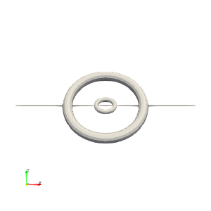
Agent Result

📏 Vision Evaluation Rubrics

Score Summary

Total Score

33/40

Goals

4

Points/Goal

10

Goal 1

9/10

Criterion: GLTF Import Success: Are the specified GLTF nodes properly imported and displayed as separate geometric components?

Judge's Assessment: Ground truth shows a GLTF import consisting of ring-like geometry plus a thin axle/rod passing horizontally through the center. The result image shows the same overall set of components rendered correctly as 3D geometry, indicating the import succeeded. Minor differences in shading/background compared to GT prevent a perfect match.

Goal 2

9/10

Criterion: Node Selection: Are all three specified nodes (Axle, Torus002, InnerRing) correctly imported and visible?

Judge's Assessment: All three expected parts appear present: (1) the long thin axle/rod spanning left-right, (2) the large outer ring (Torus002), and (3) the smaller inner ring at the center (InnerRing). Their relative placement matches the GT well; any discrepancies are subtle (primarily rendering/appearance rather than missing geometry).

Goal 3

8/10

Criterion: Camera Positioning: Is the camera positioned in the positive Y direction with appropriate zoom to fit all imported geometry? Carefully compare the camera position of GT and result images.

Judge's Assessment: The camera orientation and framing are very similar (axle horizontal, rings centered, zoom-to-fit). However, compared to the GT the perspective/lighting appears slightly different, suggesting a small mismatch in camera parameters or view settings (still clearly from the intended direction and fit).

Goal 4

7/10

Criterion: Layout Configuration: Is the view properly sized to 300x300 pixels with correct rendering and background palette?

Judge's Assessment: The result appears to be 300x300 like the GT, and the view is properly rendered. However, the background palette does not match the GT set: one GT view is white and another is a BlueGray background, while the result shown uses the darker blue-gray background only, indicating a mismatch in palette/application or view/background configuration relative to the expected ground-truth image(s).

Overall Assessment

The result largely matches the ground truth in terms of imported GLTF geometry, correct node visibility, and overall camera framing. The main deviations are in background/palette consistency and small rendering/camera/lighting differences, so it is a strong but not perfect match.

📊 Detailed Metrics

Visualization Quality

33/40

Output Generation

5/5

Efficiency

8/10

Completed in 128.34 seconds (good)

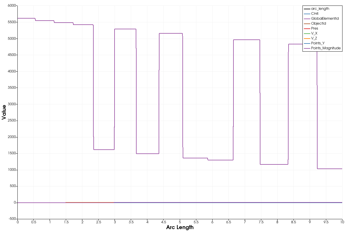
📝 line-plot

33/55 (60.0%)

📋 Task Description

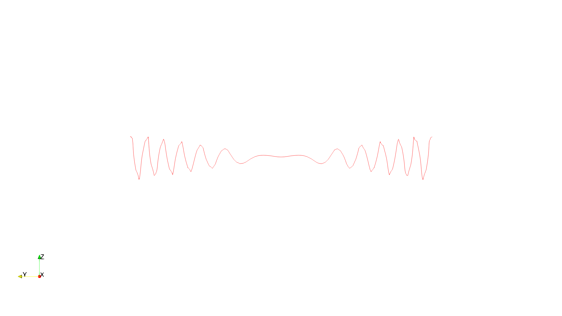
Read the dataset in the file "line-plot/data/line-plot.ex2", and print the number of components and the range of all the variables. Show a default view of the dataset, colored by the variable Pres. Create a line plot over all the variables in the dataset, from (0,0,0) to (0,0,10). Write the values of the line plot in the file "line-plot/results/{agent_mode}/line-plot.csv", and save a screenshot of the line plot in "line-plot/results/{agent_mode}/line-plot.png". (Optional, but must save if use paraview) Save the paraview state as "line-plot/results/{agent_mode}/line-plot.pvsm". (Optional, but must save if use python script) Save the python script as "line-plot/results/{agent_mode}/line-plot.py". Do not save any other files, and always save the visualization image.

🖼️ Visualization Comparison

Ground Truth

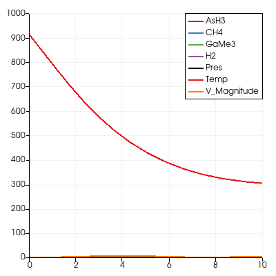
Agent Result

📏 Vision Evaluation Rubrics

Score Summary

Total Score

19/40

Goals

4

Points/Goal

10

Goal 1

6/10

Criterion: Line Visualization Quality: Are multiple distinct lines clearly visible and properly rendered showing the evolution of different variables along the specified path?

Judge's Assessment: Ground truth shows multiple variable curves along the 0–10 line, with Pres/Temp clearly varying while others sit near zero. The result image does contain multiple plotted series, but the plot is dominated by a large step-like curve (purple) and most other lines are compressed near y≈0, making the intended multi-variable evolution much less clearly visible than in the ground truth.

Goal 2

4/10

Criterion: Variable Differentiation: Are all dataset variables visually distinguishable through distinct colors or line styles with clear separation between curves?

Judge's Assessment: In the ground truth, variables are differentiated with distinct colors and a concise legend (AsH3, CH4, GaMe3, H2, Pres, Temp, V_Magnitude). In the result, the legend includes different/unexpected variables (e.g., GlobalElementId, ObjectId, V_X, V_Z, Points_Y, Points_Magnitude), and many lines overlap at the bottom due to scale, so variables are not as distinctly separable as in the ground truth.

Goal 3

3/10

Criterion: Axis and Scale Appropriateness: Do the plot axes display appropriate ranges and scaling that effectively show the data trends and variations?

Judge's Assessment: Ground truth uses an axis range (~0–1000) appropriate to show Pres/Temp trends while keeping other variables visible near zero. The result uses a much larger y-range (up to ~6000 with negatives), driven by the step-like series, which flattens most other variables and obscures their trends compared to the ground truth.

Goal 4

6/10

Criterion: Legend and Readability: Is there a clear legend identifying each variable line with readable labels and proper visual organization?

Judge's Assessment: Both images include a legend in the upper-right and the axes are labeled. However, the result legend is longer, includes different variable names than the ground truth, and readability/interpretability suffers because the key variables from the expected plot are not clearly the ones being shown or emphasized.

Overall Assessment

The result produces a line plot with multiple series and a legend, but it does not visually match the expected ground-truth plot: the set of variables differs, the y-axis scaling is inappropriate for seeing most variables, and one dominant step-like curve overwhelms the plot. Overall, the core idea of a line plot is present, but it only partially fulfills the intended multi-variable line-plot visualization along the specified path.

📊 Detailed Metrics

Visualization Quality

19/40

Output Generation

5/5

Efficiency

9/10

Completed in 66.30 seconds (very good)

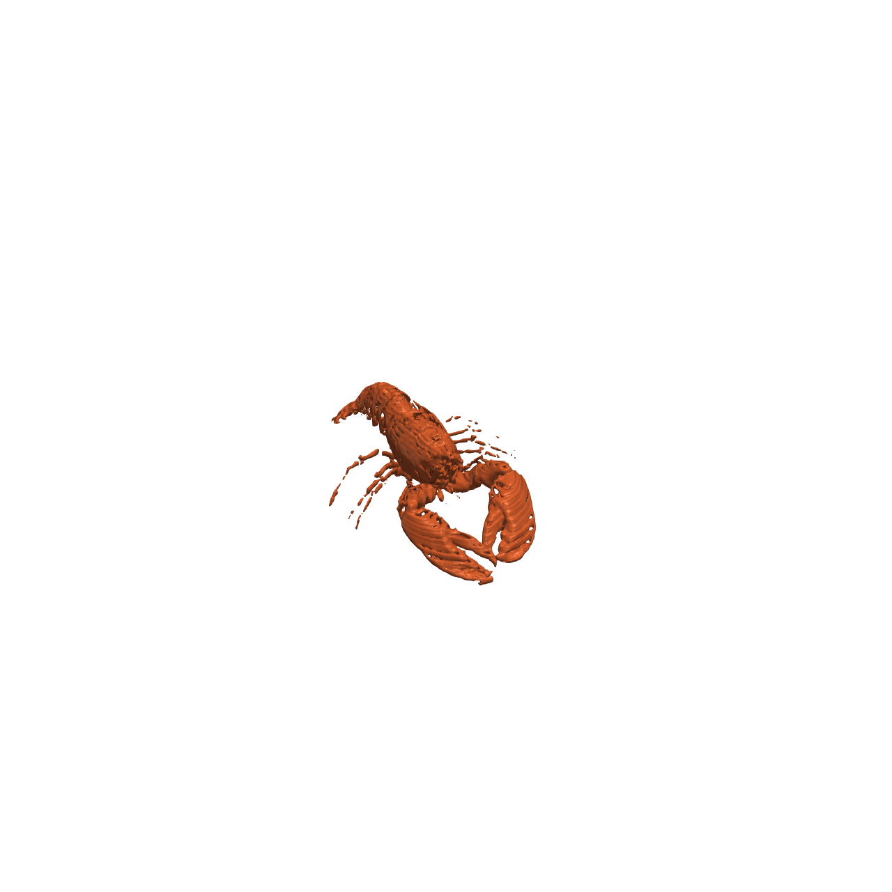
📝 lobster

32/55 (58.2%)

📋 Task Description

Task: Load the Lobster dataset from "lobster/data/lobster_301x324x56_uint8.raw", the information about this dataset: Lobster Description: CT scan of a lobster contained in a block of resin. Data Type: uint8 Data Byte Order: little Endian Data Spacing: 1x1x1.4 Data Extent: 301x324x56 Data loading is very important, make sure you correctly load the dataset according to their features. Visualize the scanned specimen: 1. Create an isosurface at the specimen boundary, find a proper isovalue to show the whole structure. 2. Use natural colors appropriate for the specimen (red-orange for lobster) 3. Analyze the visualization and answer the following questions: Q1: Based on the isosurface visualization of the lobster specimen, how many walking legs are visible? A. 6 walking legs B. 7 walking legs C. 8 walking legs D. 10 walking legs 4. Use a white background. Find an optimal view. Render at 1280x1280. Do not show a color bar or coordinate axes. 5. Set the viewpoint parameters as: [543.52, -957.0, 1007.87] to position; [150.0, 161.5, 38.5] to focal point; [-0.15, 0.62, 0.77] to camera up direction. 6. Save your work: Save the visualization image as "lobster/results/{agent_mode}/lobster.png". Save the answers to the analysis questions in plain text as "lobster/results/{agent_mode}/answers.txt". (Optional, but must save if use paraview) Save the paraview state as "lobster/results/{agent_mode}/lobster.pvsm". (Optional, but must save if use pvpython script) Save the python script as "lobster/results/{agent_mode}/lobster.py". (Optional, but must save if use VTK) Save the cxx code script as "lobster/results/{agent_mode}/lobster.cxx" Do not save any other files, and always save the visualization image and the text file.

🖼️ Visualization Comparison

Ground Truth

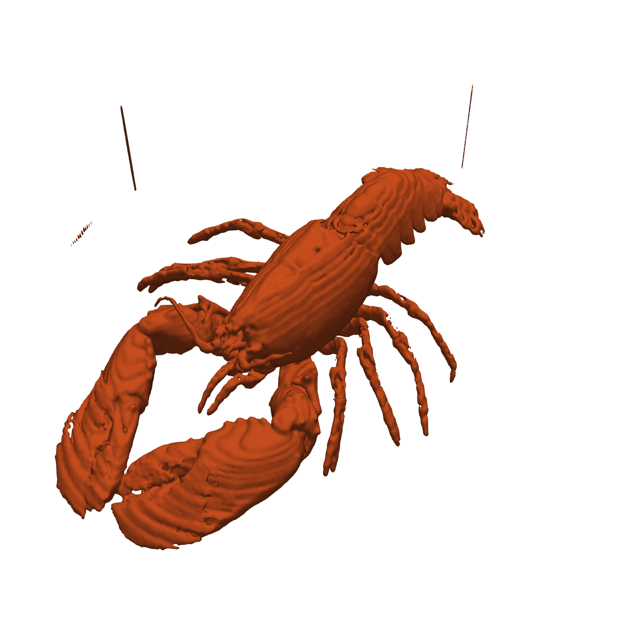
Agent Result

📏 Vision Evaluation Rubrics

Score Summary

Total Score

19/30

Goals

3

Points/Goal

10

Goal 1

5/10

Criterion: Overall Goal: Does the visualization clearly show the structure and details of the Lobster?

Judge's Assessment: The ground truth shows the lobster filling much of the frame with an optimal close view where major anatomical structures (carapace, claws, legs) are clearly visible. The result image contains the lobster but it is extremely zoomed out (tiny in the center), so the overall specimen structure and details are not readily visible at the intended scale/view, even though the object appears to be the correct dataset and isosurface.

Goal 2

6/10

Criterion: Boundary Clearity: Are surface details and boundaries of the lobster well-defined?

Judge's Assessment: In the ground truth, the isosurface boundary is crisp and surface ridges/segmentation are easy to see. In the result, the boundary seems reasonably extracted (the lobster shape is intact), but because the model is rendered very small, fine surface details and boundary clarity are effectively lost; additionally, thin appendages look less legible at that scale.

Goal 3

8/10

Criterion: Correct Color: Is the color of the lobster mimic a real one? (red-orange)

Judge's Assessment: Both images use an appropriate red-orange lobster-like color on a white background. The result’s hue is close to the ground truth, with only minor differences in shading/lighting that do not strongly affect the perceived natural coloration.

Overall Assessment

The result appears to have the correct isosurface and an appropriate red-orange color on a white background, but it fails to match the ground truth’s optimal viewpoint/framing: the lobster is rendered far too small, which substantially reduces visibility of structural detail and boundary definition.

📝 Text-Based Q&A Evaluation

Score

0/10 (0.0%)

Questions & Correct Answers

1. Q1 correct answer: B. 7 walking legs

Agent's Answers

Q1: Based on the isosurface visualization of the lobster specimen, how many walking legs are visible?
Answer: C. 8 walking legs

Explanation: In the visualization from the specified viewpoint, 8 walking legs are clearly visible - 4 on each side of the lobster's body. The lobster's two large claws (chelipeds) are also visible at the front, which along with the 8 walking legs make up the lobster's 10 total legs.

Judge's Evaluation

Evaluation:

Criterion 1 (Q1 correct answer: B. 7 walking legs): The provided answer selects C (8 walking legs), which directly contradicts the evaluation criterion stating the correct answer is 7. The explanation reinforces the incorrect count by asserting 4 legs per side are clearly visible and discussing the lobster’s total of 10 legs including claws, but this does not align with the required visible walking-leg count of 7 from the specified viewpoint. Because the core requirement is the correct visible walking-leg number, and the answer is wrong, it does not meet the criterion.

📊 Detailed Metrics

Visualization Quality

19/30

Output Generation

5/5

Efficiency

8/10

Completed in 100.20 seconds (good)

PSNR

21.42 dB

SSIM

0.9441

LPIPS

0.0601

Text Q&A Score

0/10

0.0%

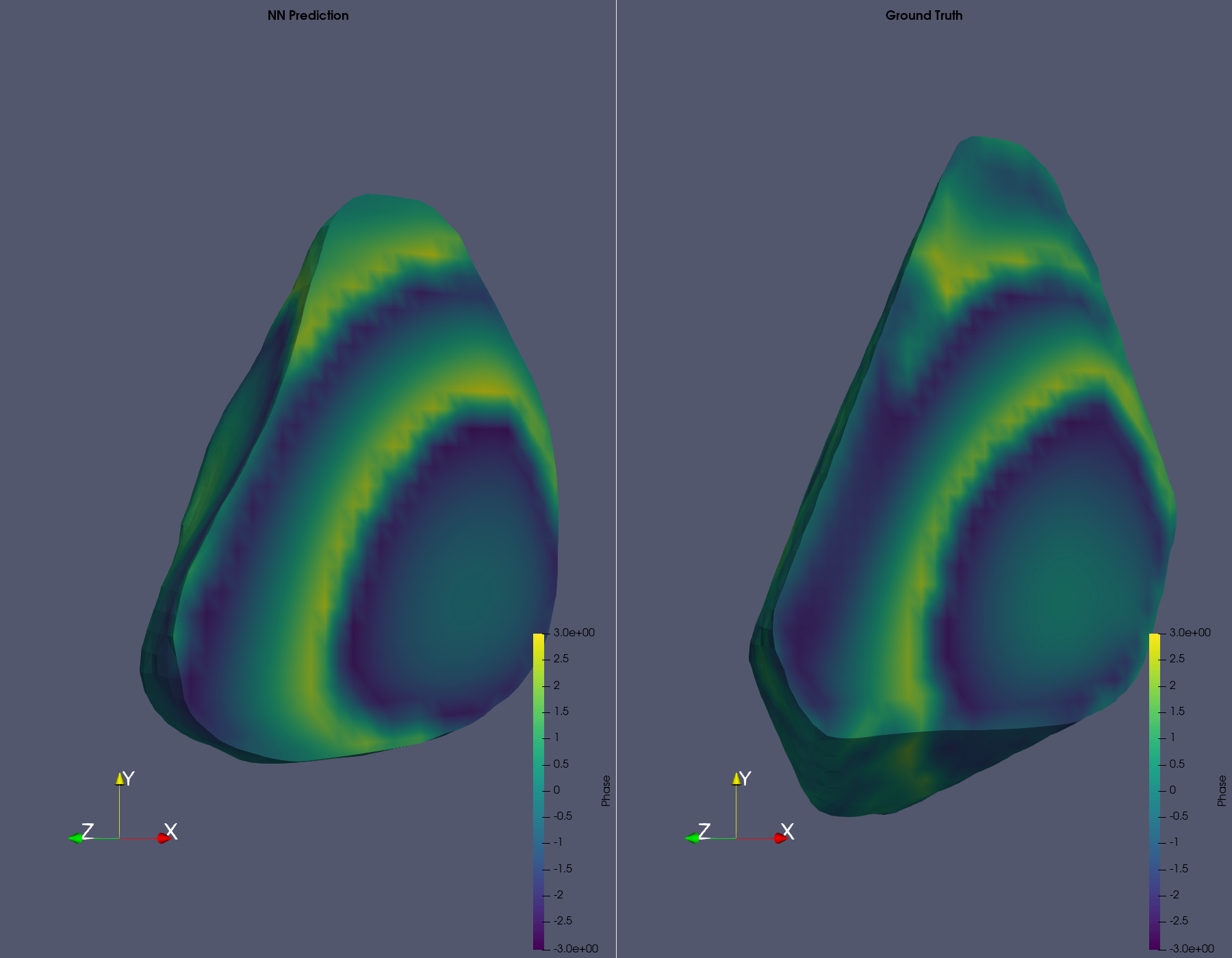
📝 materials

51/55 (92.7%)

📋 Task Description

Compare two datasets in two views side by side each 900 pixels wide x 1400 pixels high. Read the dataset "materials/data/materials_prediction.vtr" in the left view and "materials/data/materials_ground_truth.vtr" in the right view. In both views, convert the "Intensity" and "Phase" variables from cell to point data. In both views, take an isovolume of the "Intensity" variable in the range of [0.2, 1.0], clipped with a plane at (32.0, 32.0, 32.0) and +x normal direction. Color both views with the Viridis (matplotlib) color map for the "Phase" variable, scaled to the data range, including a colormap legend in both views. Label the left view "NN Prediction" and the right view "Ground Truth". Orient the camera to look in the (-1, 0, -1) direction, with the datasets fitting in the views. Save the visualization image as "materials/results/{agent_mode}/materials.png". (Optional, but must save if use paraview) Save the paraview state as "materials/results/{agent_mode}/materials.pvsm". (Optional, but must save if use python script) Save the python script as "materials/results/{agent_mode}/materials.py". Do not save any other files, and always save the visualization image.

🖼️ Visualization Comparison

Ground Truth

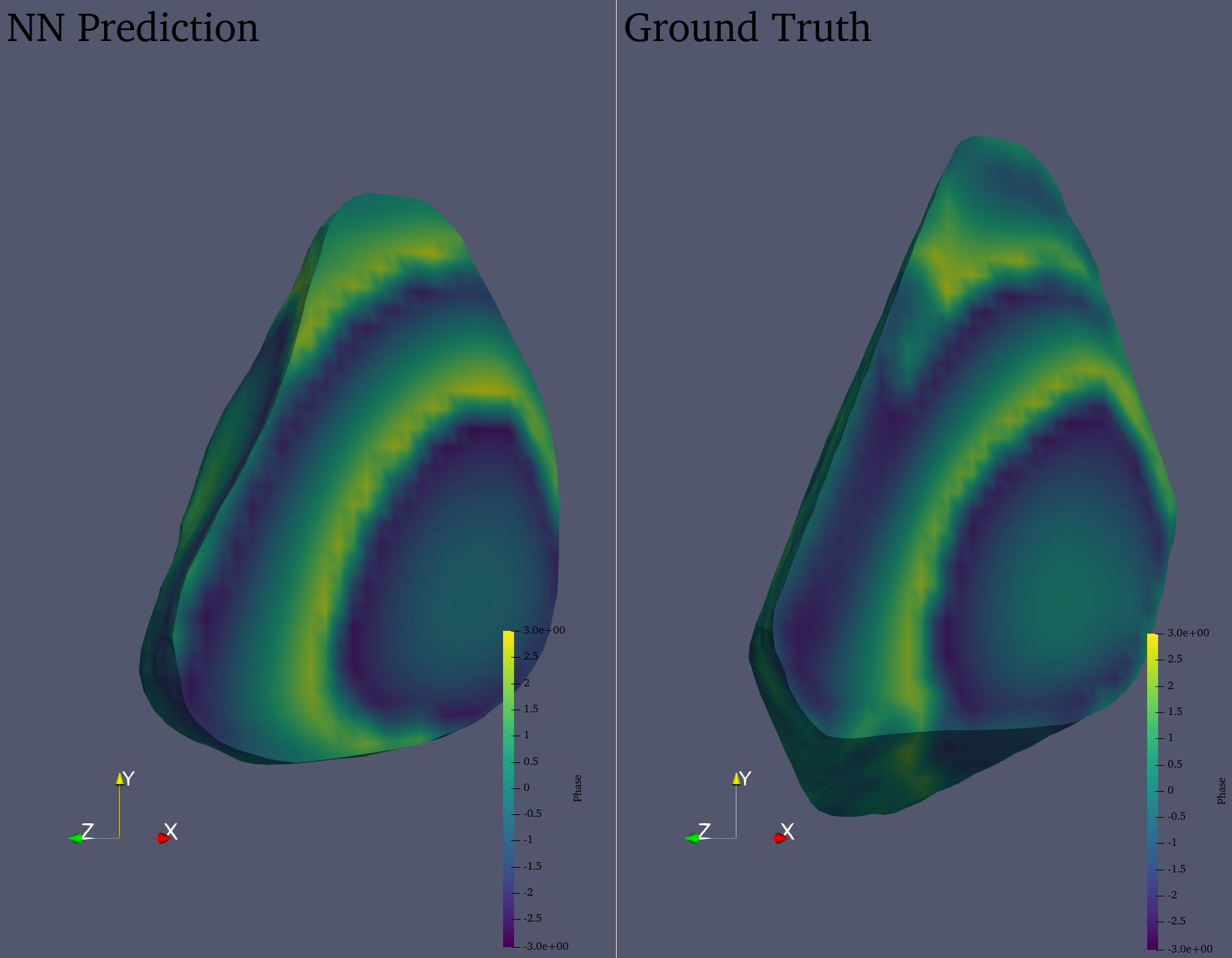
Agent Result

📏 Vision Evaluation Rubrics

Score Summary

Total Score

38/40

Goals

4

Points/Goal

10

Goal 1

10/10

Criterion: Side-by-Side Comparison: Are both datasets properly displayed in side-by-side views with correct dimensions and labeling?

Judge's Assessment: Result matches the ground truth layout: two side-by-side views separated by a vertical divider, left labeled "NN Prediction" and right labeled "Ground Truth". The objects occupy similar screen space in each panel and appear rendered at the expected aspect for the combined image.

Goal 2

9/10

Criterion: Data Conversion and Filtering: Are the Intensity and Phase variables correctly converted to point data and isovolume filtering applied?

Judge's Assessment: The extracted geometry in both panels closely matches the ground truth isovolume appearance (same overall blob shape and internal banding), indicating the Intensity isovolume range and the use of point-interpolated Phase are likely correct. Minor potential differences are not visually apparent, so only a small uncertainty remains about the exact cell-to-point conversion and threshold range fidelity.

Goal 3

9/10

Criterion: Clipping and Color Mapping: Is the plane clipping correctly applied and Viridis colormap properly used for Phase variable?

Judge's Assessment: Coloring matches Viridis-like progression (purple/blue to green/yellow) and both panels include a Phase color legend with the same approximate range and labeling. The clipped shape looks consistent with a planar cut (flat-ish truncation visible), though the plane position/orientation cannot be verified beyond visual similarity; overall it matches the ground truth very closely.

Goal 4

10/10

Criterion: Camera and Layout: Is the camera positioned correctly in (-1, 0, -1) direction with appropriate fitting and legends visible?

Judge's Assessment: Camera/view direction and zoom match the ground truth: both objects are viewed from the same (-1,0,-1)-like oblique direction, fit well within each panel, and the orientation triads and legends are visible and positioned consistently.

Overall Assessment

The result image is effectively identical to the provided ground truth: correct side-by-side setup with labels, matching isovolume/clipped geometry, Viridis Phase coloring with legends in both views, and consistent camera framing. Only negligible uncertainty remains in confirming exact filter parameters from visuals alone.

📊 Detailed Metrics

Visualization Quality

38/40

Output Generation

5/5

Efficiency

8/10

Completed in 133.77 seconds (good)

📝 mhd-magfield_streamribbon

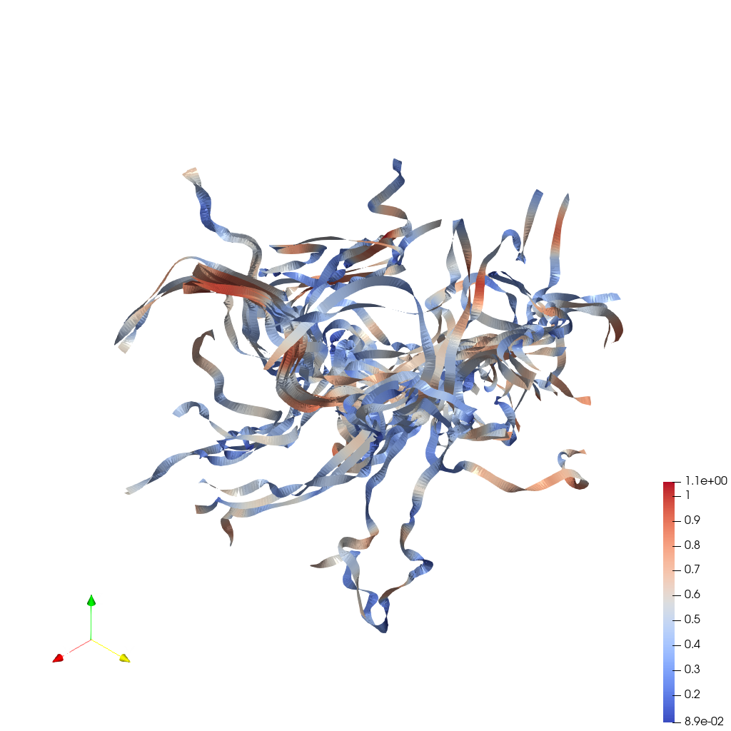
48/55 (87.3%)

📋 Task Description

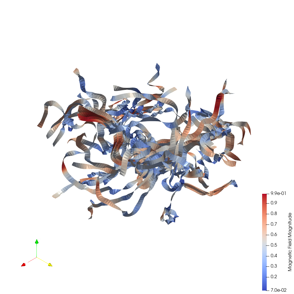
Load the MHD magnetic field dataset from "mhd-magfield_streamribbon/data/mhd-magfield_streamribbon.vti" (VTI format, 128x128x128 grid with components bx, by, bz). Generate a stream ribbon seeded from a line source along the y-axis at x=64, z=64 (from y=20 to y=108), with 30 seed points. The stream ribbon should be traced along the magnetic field lines. Color the stream ribbon by magnetic field magnitude using the 'Cool to Warm' colormap. Enable surface lighting with specular reflection for better 3D perception. Add a color bar labeled 'Magnetic Field Magnitude'. Use a white background. Set an isometric camera view. Render at 1024x1024 resolution. Set the viewpoint parameters as: [200.0, 200.0, 200.0] to position; [63.5, 63.5, 63.5] to focal point; [0.0, 0.0, 1.0] to camera up direction. Save the visualization image as "mhd-magfield_streamribbon/results/{agent_mode}/mhd-magfield_streamribbon.png". (Optional, but must save if use paraview) Save the paraview state as "mhd-magfield_streamribbon/results/{agent_mode}/mhd-magfield_streamribbon.pvsm". (Optional, but must save if use pvpython script) Save the python script as "mhd-magfield_streamribbon/results/{agent_mode}/mhd-magfield_streamribbon.py". (Optional, but must save if use VTK) Save the cxx code script as "mhd-magfield_streamribbon/results/{agent_mode}/mhd-magfield_streamribbon.cxx" Do not save any other files, and always save the visualization image.

🖼️ Visualization Comparison

Ground Truth

Agent Result

📏 Vision Evaluation Rubrics

Score Summary

Total Score

35/40

Goals

4

Points/Goal

10

Goal 1

9/10

Criterion: Overall Visualization Goal: Does the result match the ground truth stream ribbon visualization of the MHD magnetic field?

Judge's Assessment: The result shows a dense cluster of stream ribbons on a white background with an isometric-like view, surface lighting, and a cool-to-warm style diverging colormap plus a vertical color bar. Overall composition strongly matches the ground truth. Minor differences include slightly different color bar range/formatting (ground truth tops near 1.1e+00 vs result near 9.9e-01) and small variations in ribbon placement/orientation suggesting seeding/integration/camera not perfectly identical.

Goal 2

9/10

Criterion: Surface Patterns: Does the stream ribbon show similar flow patterns and structures as the ground truth?

Judge's Assessment: The ribbon flow patterns (tangled, ribbon-like trajectories with similar curling and branching behavior) are very close to the ground truth. The central knot and outward-splaying ribbons appear in similar locations, with only subtle differences in a few ribbon paths and local twisting that don’t change the overall structure.

Goal 3

9/10

Criterion: Surface Coverage: Is the spatial extent and shape of the stream ribbon similar to the ground truth?

Judge's Assessment: Spatial extent and coverage are highly similar: the ribbon bundle occupies the same central volume and spreads to comparable left/right/top regions. A few ribbons extend slightly differently (e.g., some right-side and lower-center elements), but the overall envelope/shape matches well.

Goal 4

8/10

Criterion: Color Mapping: Is the color distribution across the surface visually similar to the ground truth?

Judge's Assessment: Color distribution is broadly similar (dominant blues with intermittent warm orange/red segments in comparable regions). However, the result shows slightly different intensity scaling and warm-color prominence in a few ribbons (notably some stronger reds), consistent with a different magnitude range/normalization compared to the ground truth color bar.

Overall Assessment

The result is an excellent match to the expected MHD stream-ribbon visualization: correct type of geometry, similar flow structures and coverage, white background, and appropriate cool-to-warm magnitude coloring with a labeled color bar. Small discrepancies are mainly in color scaling and minor ribbon/camera/integration differences.

📊 Detailed Metrics

Visualization Quality

35/40

Output Generation

5/5

Efficiency

8/10

Completed in 92.65 seconds (good)

PSNR

17.13 dB

SSIM

0.8723

LPIPS

0.1332

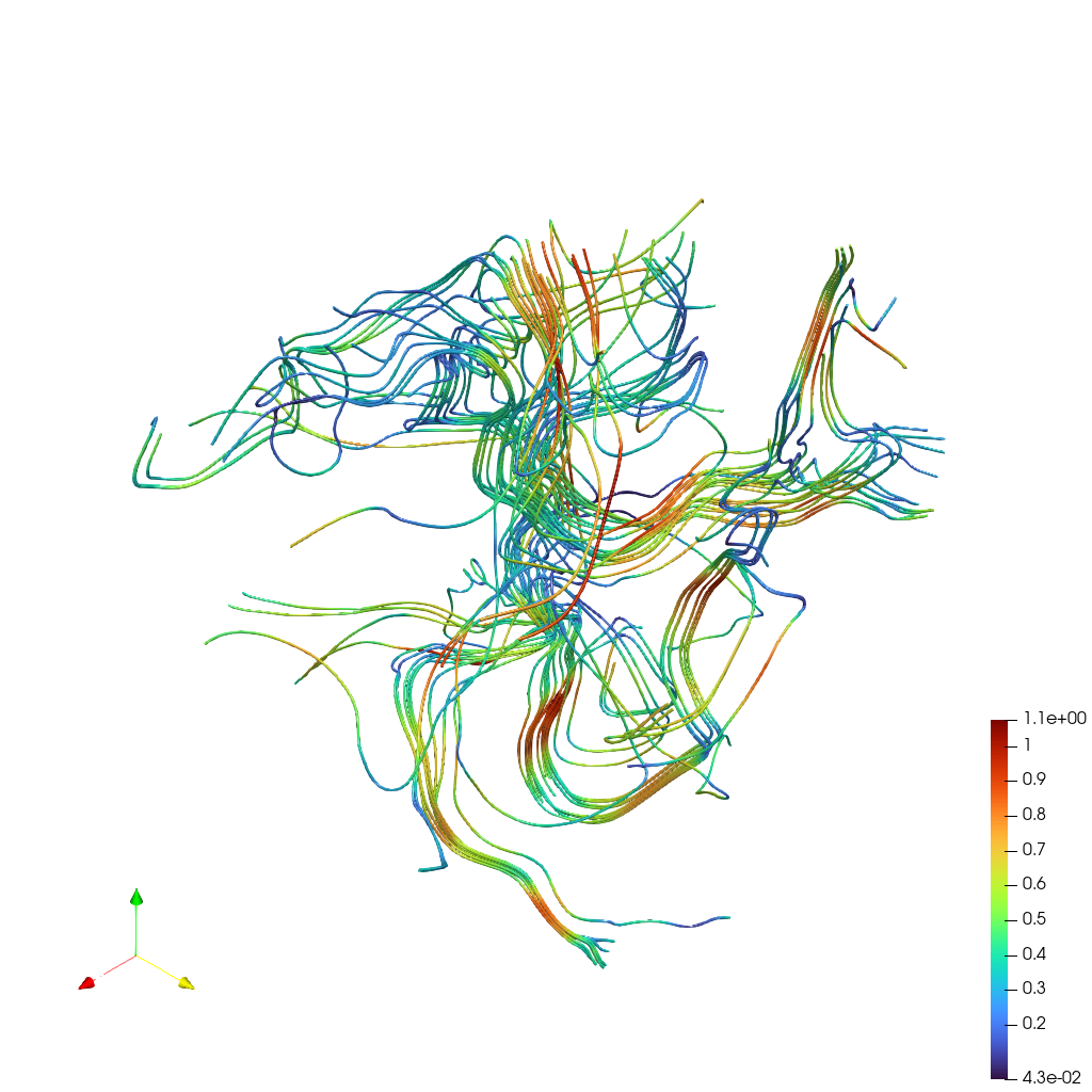
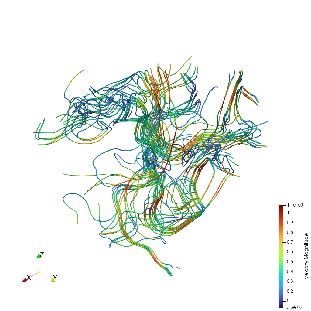
📝 mhd-turbulence_pathline

45/55 (81.8%)

📋 Task Description

Load the MHD turbulence velocity field time series "mhd-turbulence_pathline/data/mhd-turbulence_pathline_{timestep}.vti", where "timestep" in {0000, 0010, 0020, 0030, 0040} (5 timesteps, VTI format, 128x128x128 grid each). Compute true pathlines by tracking particles through the time-varying velocity field using the ParticlePath filter. Apply TemporalShiftScale (scale=20) and TemporalInterpolator (interval=0.5) to extend particle travel and smooth trajectories. Seed 26 points along a line on the z-axis at x=64, y=64 (from z=20 to z=108). Use static seeds with termination time 80. 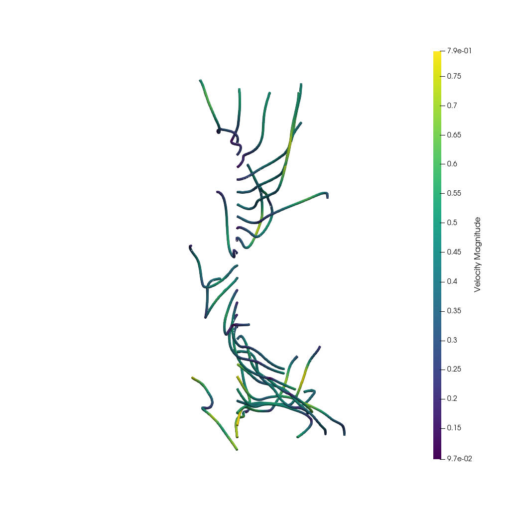Render pathlines as tubes with radius 0.3. Color by velocity magnitude using the 'Viridis (matplotlib)' colormap. Add a color bar for velocity magnitude. Set the viewpoint parameters as: [200.0, 200.0, 200.0] to position; [63.5, 63.5, 63.5] to focal point; [0.0, 0.0, 1.0] to camera up direction. Use a white background. Set an isometric camera view. Render at 1024x1024. Save the visualization image as "mhd-turbulence_pathline/results/{agent_mode}/mhd-turbulence_pathline.png". (Optional, but must save if use paraview) Save the paraview state as "mhd-turbulence_pathline/results/{agent_mode}/mhd-turbulence_pathline.pvsm". (Optional, but must save if use pvpython script) Save the python script as "mhd-turbulence_pathline/results/{agent_mode}/mhd-turbulence_pathline.py". (Optional, but must save if use VTK) Save the cxx code script as "mhd-turbulence_pathline/results/{agent_mode}/mhd-turbulence_pathline.cxx" Do not save any other files, and always save the visualization image.

🖼️ Visualization Comparison

Ground Truth

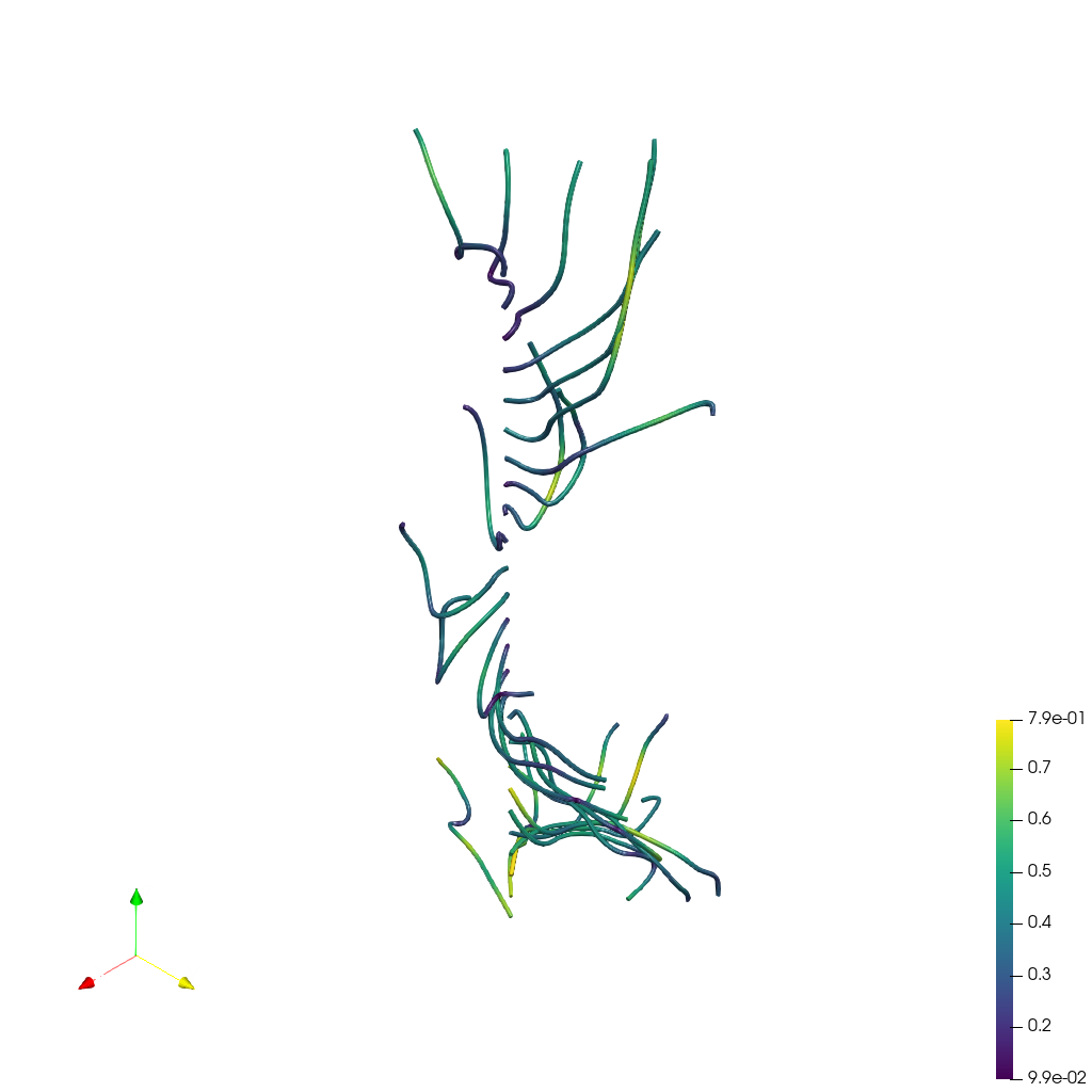
Agent Result

📏 Vision Evaluation Rubrics

Score Summary

Total Score

35/40

Goals

4

Points/Goal

10

Goal 1

9/10

Criterion: Overall Visualization Goal: Does the result match the ground truth pathline visualization of the MHD turbulence velocity field?

Judge's Assessment: The result image closely matches the ground truth: white background, isometric view, tubular pathlines, and a Viridis-colored velocity magnitude legend on the right. Composition and camera framing are essentially the same, with only minor presentation differences (colorbar formatting/labeling and slightly different tick placement).

Goal 2

9/10

Criterion: Pathline Patterns: Do the pathlines show similar particle trajectories and flow structures as the ground truth?

Judge's Assessment: The pathline trajectories show the same overall turbulent structures as the ground truth: a tall, vertically-elongated bundle with similar curvature, crossing strands in the midsection, and a denser tangle near the lower portion. Minor differences appear in a few individual strand shapes/lengths, but the dominant patterns match well.

Goal 3

9/10

Criterion: Pathline Coverage: Is the spatial extent and distribution of pathlines similar to the ground truth?

Judge's Assessment: Spatial coverage is very similar: comparable number of pathlines, similar vertical extent, and similar clustering (sparser upper region, denser lower cluster). Any discrepancies are small (a few pathlines appear slightly shifted or truncated relative to the ground truth).

Goal 4

8/10

Criterion: Color Mapping: Is the color distribution along pathlines visually similar to the ground truth?

Judge's Assessment: Color mapping appears consistent with Viridis and the same general range (purple low to yellow high). The distribution of colors along the tubes is largely similar, but the colorbar styling differs (ground truth has a more compact bar with fewer labels; result has a labeled 'Velocity Magnitude' bar and slightly different tick/endpoint formatting), and there may be slight differences in normalization endpoints (bottom value shown differs slightly).

Overall Assessment

Overall the result is an excellent match to the ground truth: camera/view, pathline geometry, and overall color appearance align closely. Differences are limited to minor per-trajectory variations and colorbar/legend formatting and scale annotation.

📊 Detailed Metrics

Visualization Quality

35/40

Output Generation

5/5

Efficiency

5/10

Completed in 324.42 seconds (very slow)

PSNR

17.77 dB

SSIM

0.9420

LPIPS

0.1814

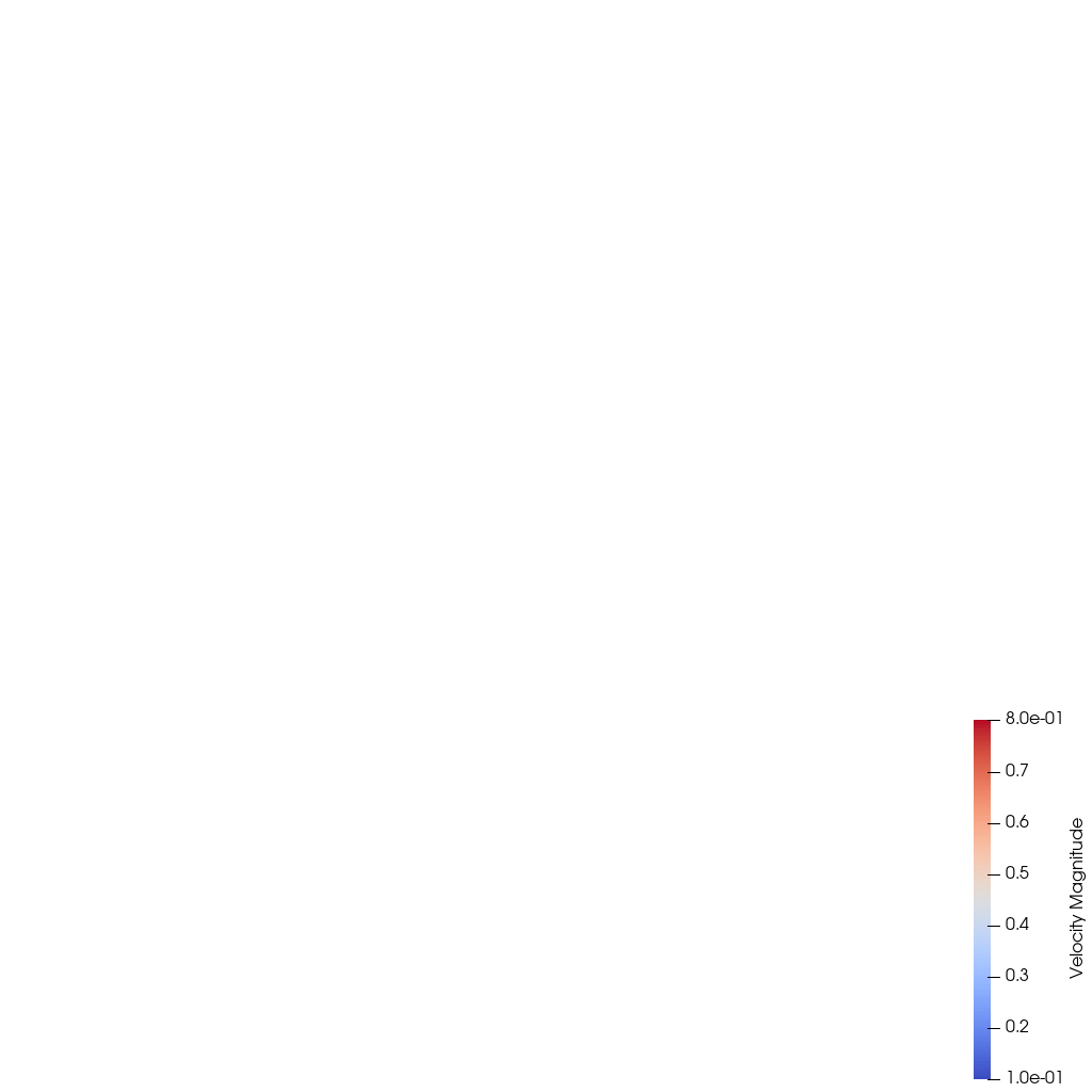
📝 mhd-turbulence_pathribbon

❌ FAILED

0/45 (0.0%)

📋 Task Description

Load the MHD turbulence velocity field time series "mhd-turbulence_pathribbon/data/mhd-turbulence_pathribbon_{timestep}.vti", where "timestep" in {0000, 0010, 0020, 0030, 0040} (5 timesteps, VTI format, 128x128x128 grid each). Compute true pathlines by tracking particles through the time-varying velocity field using the ParticlePath filter. Apply TemporalShiftScale (scale=20) and TemporalInterpolator (interval=0.1) for dense, smooth trajectories. Seed 26 points along a line on the z-axis at x=64, y=64 (from z=20 to z=108). Use static seeds with termination time 80. Create ribbon surfaces from the pathlines using the Ribbon filter with width 1.5 and a fixed default normal to prevent twisting. Apply Smooth filter (500 iterations) and generate surface normals for smooth shading. Set surface opacity to 0.85. Color by velocity magnitude using the 'Cool to Warm' colormap (range 0.1-0.8). Add specular highlights (0.5). Add a color bar for velocity magnitude. Use a white background. Set an isometric camera view. Render at 1024x1024. Set the viewpoint parameters as: [200.0, 200.0, 200.0] to position; [63.5, 63.5, 63.5] to focal point; [0.0, 0.0, 1.0] to camera up direction. Save the visualization image as "mhd-turbulence_pathribbon/results/{agent_mode}/mhd-turbulence_pathribbon.png". (Optional, but must save if use paraview) Save the paraview state as "mhd-turbulence_pathribbon/results/{agent_mode}/mhd-turbulence_pathribbon.pvsm". (Optional, but must save if use pvpython script) Save the python script as "mhd-turbulence_pathribbon/results/{agent_mode}/mhd-turbulence_pathribbon.py". (Optional, but must save if use VTK) Save the cxx code script as "mhd-turbulence_pathribbon/results/{agent_mode}/mhd-turbulence_pathribbon.cxx" Do not save any other files, and always save the visualization image.

🖼️ Visualization Comparison

Ground Truth

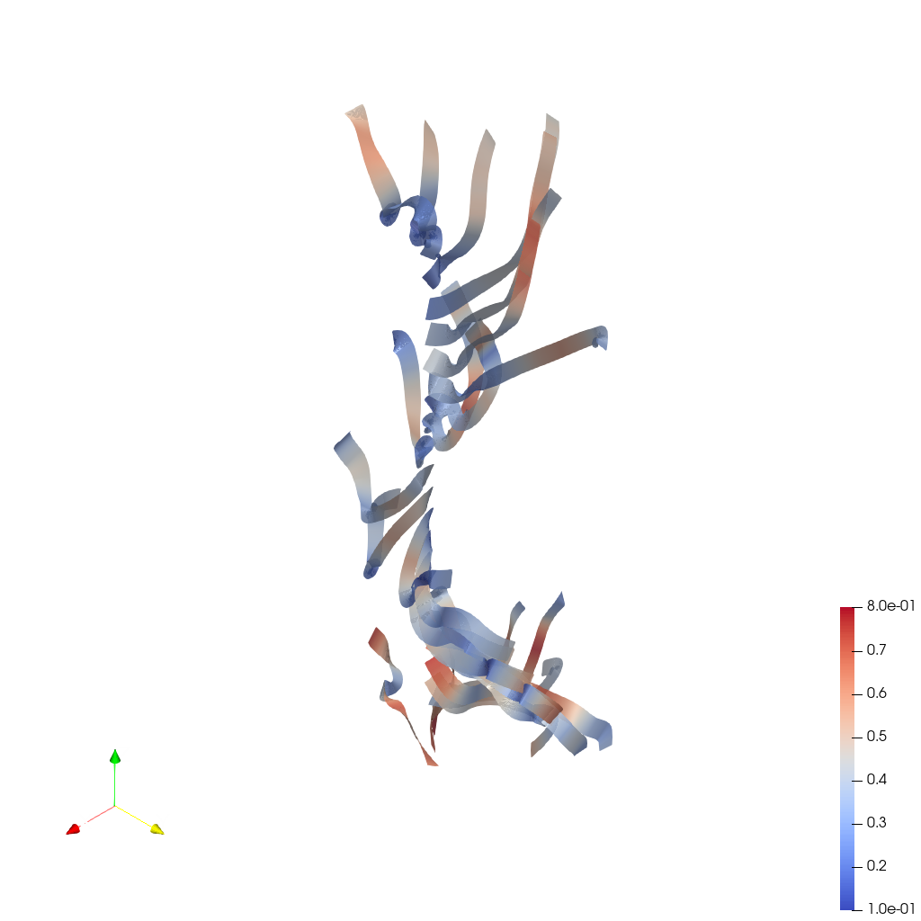
Agent Result

📏 Vision Evaluation Rubrics

Score Summary

Total Score

0/30

Goals

3

Points/Goal

10

Goal 1

1/10

Criterion: Surface Patterns: Does the path ribbon show similar flow patterns and structures as the ground truth?

Judge's Assessment: Ground truth shows a complex set of twisting path-ribbons with clear turbulent swirling/looping structures. The result image contains no visible ribbons or flow structures at all (blank white render area), so the surface patterns are not reproduced.

Goal 2

0/10

Criterion: Surface Coverage: Is the spatial extent and shape of the path ribbon similar to the ground truth?

Judge's Assessment: Ground truth has ribbons occupying a tall vertical region near the center of the domain. The result shows no geometry, hence no spatial extent/coverage can be compared; the intended ribbon surfaces are missing.

Goal 3

2/10

Criterion: Color Mapping: Is the color distribution across the surface visually similar to the ground truth?

Judge's Assessment: Ground truth displays a cool-to-warm velocity-magnitude coloration on the ribbons with a corresponding color bar. The result has only the color bar present (similar range/labeling), but since the ribbons are absent there is no color distribution on surfaces to match.

Overall Assessment

The submitted result appears to have rendered only the background and scalar bar, with the path-ribbon geometry missing/fully invisible. Consequently, flow patterns and surface coverage do not match the ground truth, and color mapping cannot be assessed on the surfaces.

📊 Detailed Metrics

Visualization Quality

3/30

Output Generation

5/5

Efficiency

5/10

Completed in 2187.97 seconds (very slow)

PSNR

23.66 dB

SSIM

0.9815

LPIPS

0.0567

📝 mhd-turbulence_streamline

48/55 (87.3%)

📋 Task Description

Load the MHD turbulence velocity field dataset "mhd-turbulence_streamline/data/mhd-turbulence_streamline.vti" (VTI format, 128x128x128 grid). Generate 3D streamlines seeded from a line source along the z-axis at x=64, y=64 (from z=0 to z=127), with 50 seed points. Color the streamlines by velocity magnitude using the 'Turbo' colormap. Set streamline tube radius to 0.3 using the Tube filter. Add a color bar labeled 'Velocity Magnitude'. Use a white background. Set an isometric camera view. Render at 1024x1024. Set the viewpoint parameters as: [200.0, 200.0, 200.0] to position; [63.5, 63.5, 63.5] to focal point; [0.0, 0.0, 1.0] to camera up direction. Save the visualization image as "mhd-turbulence_streamline/results/{agent_mode}/mhd-turbulence_streamline.png". (Optional, but must save if use paraview) Save the paraview state as "mhd-turbulence_streamline/results/{agent_mode}/mhd-turbulence_streamline.pvsm". (Optional, but must save if use pvpython script) Save the python script as "mhd-turbulence_streamline/results/{agent_mode}/mhd-turbulence_streamline.py". (Optional, but must save if use VTK) Save the cxx code script as "mhd-turbulence_streamline/results/{agent_mode}/mhd-turbulence_streamline.cxx" Do not save any other files, and always save the visualization image.

🖼️ Visualization Comparison

Ground Truth

Agent Result

📏 Vision Evaluation Rubrics

Score Summary

Total Score

35/40

Goals

4

Points/Goal

10

Goal 1

9/10

Criterion: Overall Visualization Goal: Does the result match the ground truth streamline visualization of the MHD turbulence velocity field?

Judge's Assessment: The result shows the same overall 3D streamline/tube visualization on a white background with an isometric-like view and a velocity-magnitude colorbar. The composition (central tangled bundle with lobes extending left/right and downward) matches the ground truth very closely. Minor differences are limited to annotations: the result colorbar includes the label text and the axes triad orientation/labeling differs slightly.

Goal 2

9/10

Criterion: Streamline Patterns: Do the streamlines show similar flow patterns and structures as the ground truth?

Judge's Assessment: Streamline geometry and major structures align well with the ground truth: a dense central vertical-ish core with multiple curling filaments, a prominent right-side arc/bundle, and similar looping on the left. Small deviations in a few individual streamline paths/termination points are visible (likely integration/seed ordering or rendering differences), but the dominant flow patterns are the same.

Goal 3

9/10

Criterion: Streamline Coverage: Is the spatial distribution and density of streamlines similar to the ground truth?

Judge's Assessment: Streamline density and spatial coverage are very similar: comparable number of lines, similar clustering in the center, and similar spread into the left and right regions with a handful of longer trajectories. Any differences are subtle (slightly different presence/length of a few peripheral streamlines).

Goal 4

8/10

Criterion: Color Mapping: Is the color distribution along streamlines visually similar to the ground truth?

Judge's Assessment: The color distribution along streamlines is highly similar (blue/green dominant with localized yellow/orange/red high-magnitude segments in the center and along a few right-side strands). The colormap appears consistent with Turbo-like styling, though the exact colorbar tick range/formatting differs slightly and the result’s bar label changes the visual balance compared to the ground truth.

Overall Assessment

The result is an excellent match to the ground truth: streamline/tube shapes, spatial distribution, and velocity-magnitude coloring closely correspond. Differences are minor and mostly in colorbar/axes annotations and slight variations in a few individual streamline paths.

📊 Detailed Metrics

Visualization Quality

35/40

Output Generation

5/5

Efficiency

8/10

Completed in 155.41 seconds (good)

PSNR

17.13 dB

SSIM

0.8802

LPIPS

0.1072

📝 miranda

40/45 (88.9%)

📋 Task Description

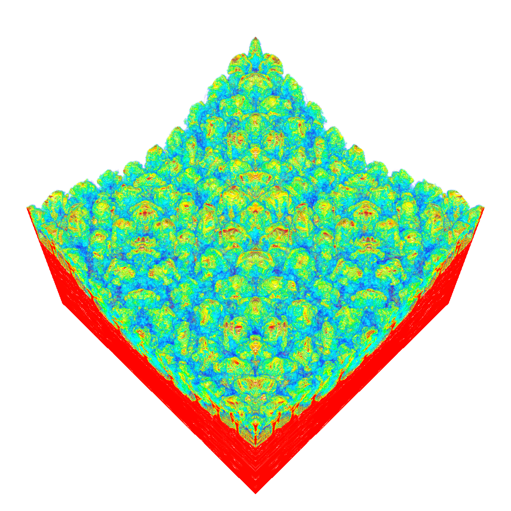
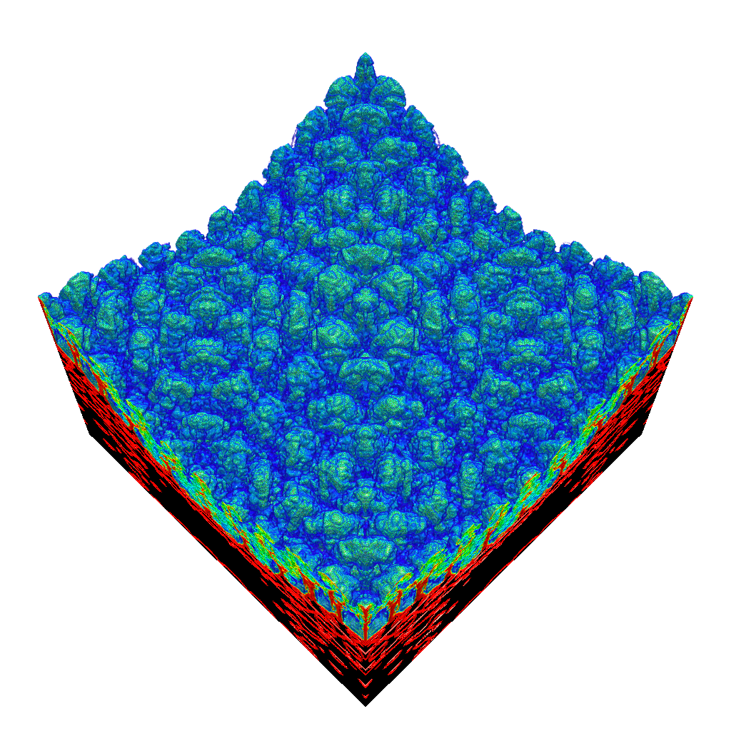
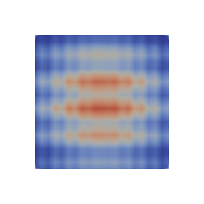
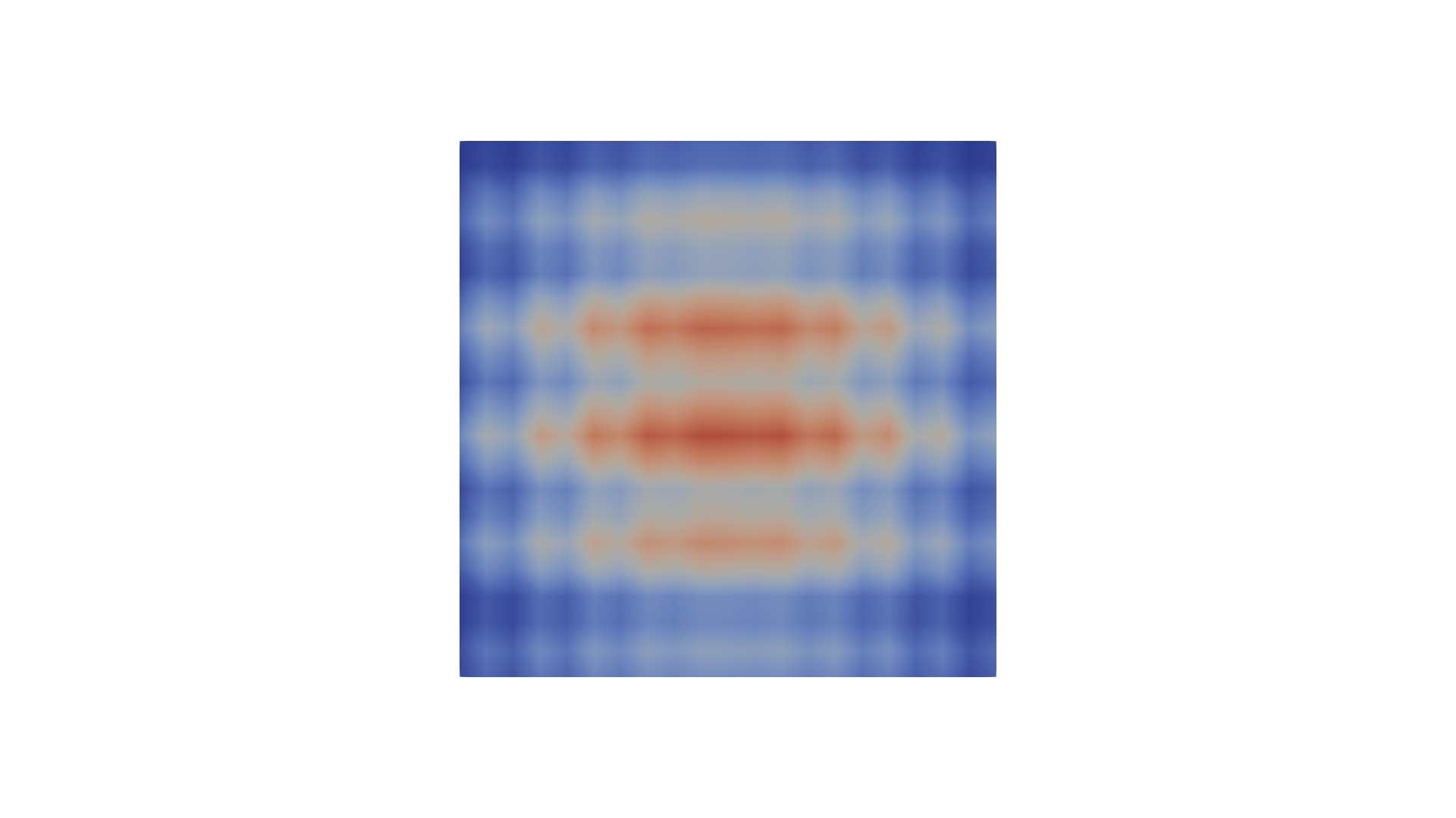
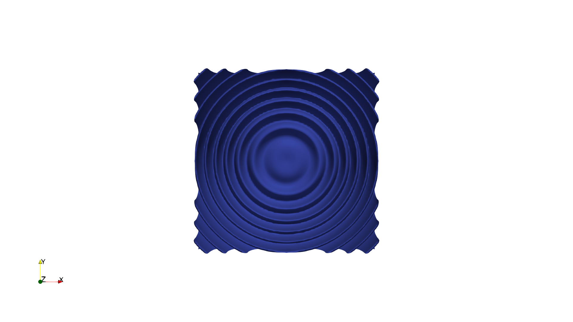
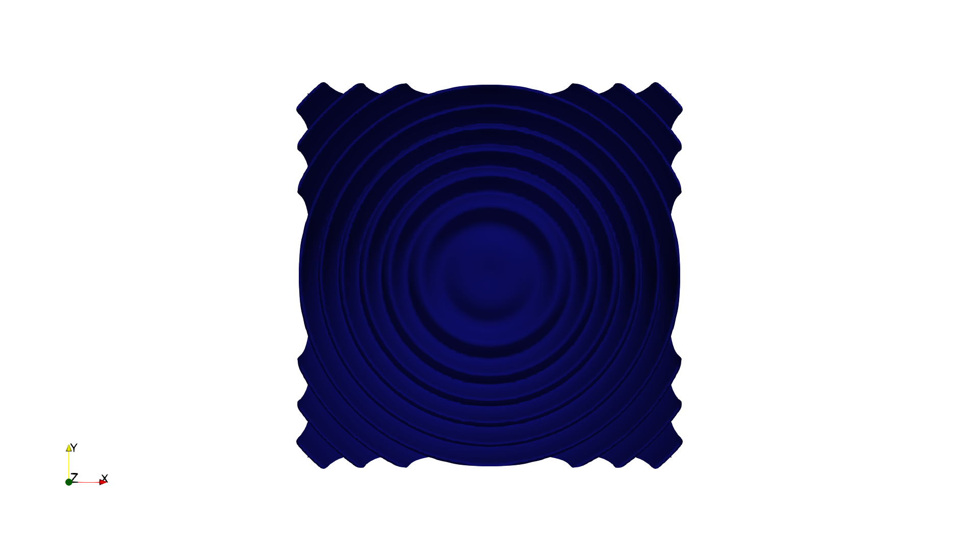
Task: Load the Rayleigh-Taylor Instability dataset from "miranda/data/miranda_256x256x256_float32.vtk". Generate a visualization image of the Rayleigh-Taylor Instability dataset, a time step of a density field in a simulation of the mixing transition in Rayleigh-Taylor instability, with the following visualization settings: 1) Create volume rendering 2) Set the opacity transfer function as a ramp function from value 0 to 1 of the volumetric data, assigning opacity 0 to value 0 and assigning opacity 1 to value 1. 3) Set the color transfer function following the 7 rainbow colors and assign a red color [1.0, 0.0, 0.0] to the highest value, a purple color [0.5, 0.0, 1.0] to the lowest value. 4) Set the viewpoint parameters as: [650, 650, 650] to position; [128, 128, 128] to focal point; [1, 0, 0] to camera up direction 5) Volume rendering ray casting sample distance is 0.1 6) White background 7) Visualization image resolution is 1024x1024 8) Don't show color/scalar bar or coordinate axes. Save the visualization image as "miranda/results/{agent_mode}/miranda.png". (Optional, but must save if use paraview) Save the paraview state as "miranda/results/{agent_mode}/miranda.pvsm". (Optional, but must save if use pvpython script) Save the python script as "miranda/results/{agent_mode}/miranda.py". (Optional, but must save if use VTK) Save the cxx code script as "miranda/results/{agent_mode}/miranda.cxx" Do not save any other files, and always save the visualization image.

🖼️ Visualization Comparison

Ground Truth

Agent Result

📏 Vision Evaluation Rubrics

Score Summary

Total Score

29/30

Goals

3

Points/Goal

10

Goal 1

10/10

Criterion: Does the visualization image clearly show the regions from low to high intensity?

Judge's Assessment: The result image matches the ground truth in overall structure and intensity mapping: low values appear in the purple/blue range, transitioning through cyan/green/yellow to orange/red for high values. The turbulent mixing features and their color distribution across the cube faces are essentially identical, clearly conveying low-to-high intensity regions.

Goal 2

9/10

Criterion: Does the purple region show areas with low opacity?

Judge's Assessment: Low-value regions (purple/blue areas, especially along the left/top portions) appear appropriately less visually dominant and more translucent compared with higher-valued regions, consistent with low opacity. Compared to the ground truth, there is at most a very slight increase in visibility/saturation of some purple areas, but the intended low-opacity effect is still preserved.

Goal 3

10/10

Criterion: Does the red region show areas with high opacity?

Judge's Assessment: High-value regions (red/orange, prominently on the right/front faces) appear strong and opaque, matching the ground truth closely. The red areas are clearly the most visually solid and dominant regions, consistent with opacity ramp assigning highest opacity to highest values.

Overall Assessment

The result is an excellent match to the ground truth: the rainbow colormap ordering and spatial distribution of intensities are effectively identical, and the opacity behavior (low values more transparent, high values more opaque) is consistent with the required ramp transfer function. Only negligible differences, if any, are visible in the low-value translucency.

📊 Detailed Metrics

Visualization Quality

29/30

Output Generation

5/5

Efficiency

6/10

Completed in 274.71 seconds (slow)

📝 ml-dvr

38/55 (69.1%)

📋 Task Description

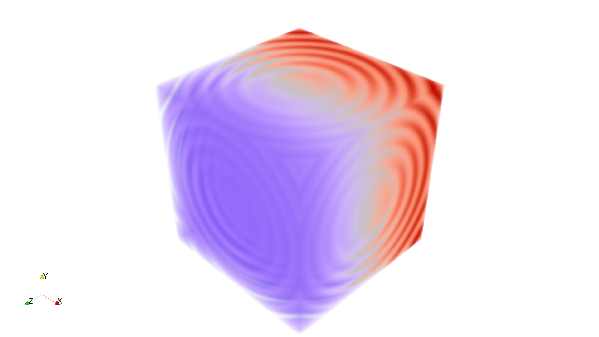
I would like to use ParaView to visualize a dataset. Read in the file named "ml-dvr/data/ml-dvr.vtk". Generate a volume rendering using the default transfer function. Rotate the view to an isometric direction. Save a screenshot of the result in the filename "ml-dvr/results/{agent_mode}/ml-dvr.png". The rendered view and saved screenshot should be 1920 x 1080 pixels. (Optional, but must save if use paraview) Save the paraview state as "ml-dvr/results/{agent_mode}/ml-dvr.pvsm". (Optional, but must save if use python script) Save the python script as "ml-dvr/results/{agent_mode}/ml-dvr.py". Do not save any other files, and always save the visualization image.

🖼️ Visualization Comparison

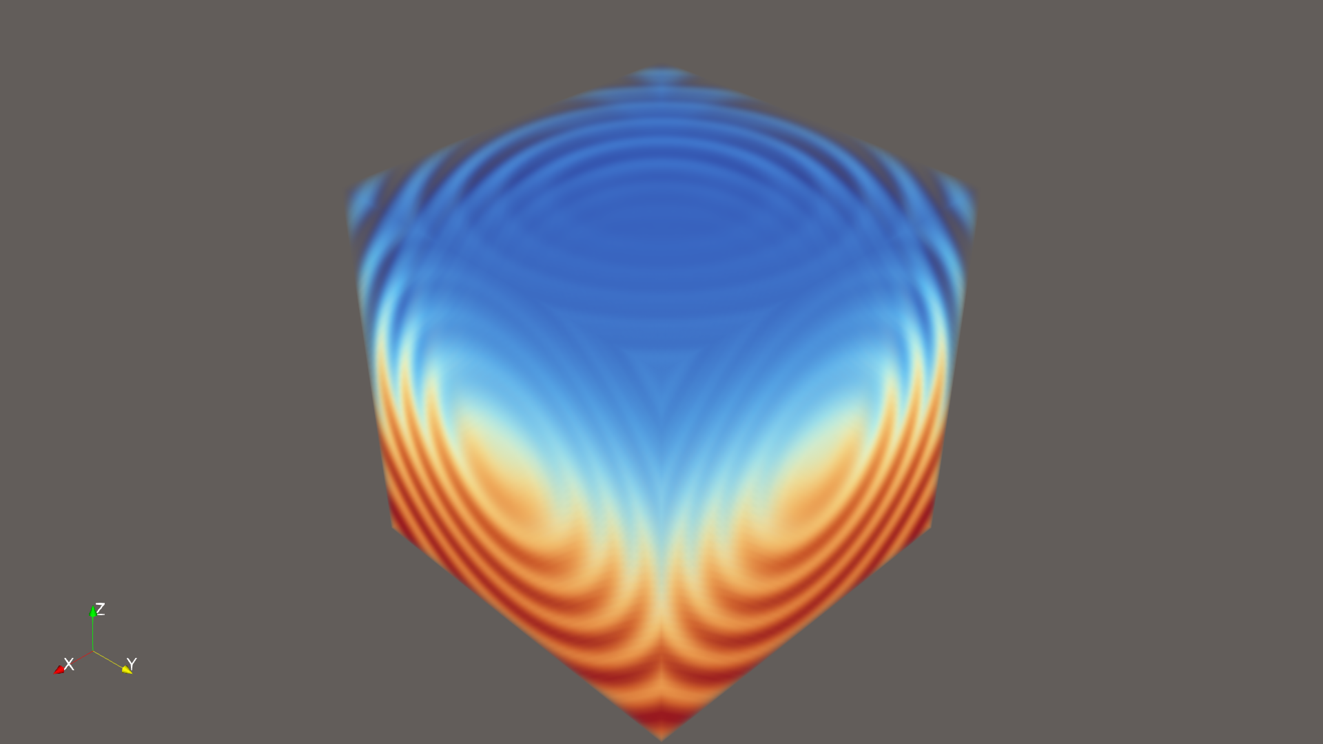
Ground Truth

Agent Result

📏 Vision Evaluation Rubrics

Score Summary

Total Score

25/40

Goals

4

Points/Goal

10

Goal 1

7/10

Criterion: Volume Rendering Quality: Is the volume rendering properly generated with appropriate opacity and color mapping that reveals internal structures?

Judge's Assessment: Both ground truth and result show a volume-rendered cube with smoothly varying internal banded/ring structures visible throughout the volume. However, the result appears more opaque and denser overall (especially in the upper half), reducing the airy/translucent look of the ground truth and slightly obscuring interior gradients.

Goal 2

5/10

Criterion: Transfer Function Application: Does the default transfer function effectively highlight meaningful data features and provide good visual contrast?

Judge's Assessment: The ground truth uses a red–purple/blue diverging look on a white background, while the result uses a blue-to-orange/yellow palette and a darker background. This indicates the transfer function (and/or color map/preset/background) does not match the expected default appearance from the ground truth, and contrast distribution across the volume differs substantially.

Goal 3

6/10

Criterion: Isometric View Setup: Is the visualization displayed from an isometric viewpoint that provides a clear three-dimensional perspective of the volume?

Judge's Assessment: Both images show a corner-forward cube consistent with an isometric-like 3D view. The result’s orientation is similar but not matching: the cube is more centered/upright with a different face emphasis compared to the ground truth’s specific isometric rotation, suggesting a different camera azimuth/elevation/roll.

Goal 4

7/10

Criterion: Visual Clarity and Detail: Are the volume details clearly visible with proper lighting and shading that enhances depth perception?

Judge's Assessment: The result has crisp banding near the lower edges and clear 3D shape cues, but the darker background and higher opacity reduce subtle interior detail and depth compared to the ground truth’s lighter, more transparent rendering where interior structures read more softly and evenly.

Overall Assessment

The submission captures the correct general volume-rendered cube with internal banding and an approximately isometric viewpoint, but it diverges notably from the ground truth in transfer function/color mapping (and background), and is somewhat more opaque, which changes the perceived internal structure and overall visual match.

📊 Detailed Metrics

Visualization Quality

25/40

Output Generation

5/5

Efficiency

8/10

Completed in 103.90 seconds (good)

📝 ml-iso

48/55 (87.3%)

📋 Task Description

Read in the file named "ml-iso/data/ml-iso.vtk", and generate an isosurface of the variable var0 at value 0.5. Use a white background color. Save a screenshot of the result, size 1920 x 1080 pixels, in "ml-iso/results/{agent_mode}/ml-iso.png". (Optional, but must save if use paraview) Save the paraview state as "ml-iso/results/{agent_mode}/ml-iso.pvsm". (Optional, but must save if use python script) Save the python script as "ml-iso/results/{agent_mode}/ml-iso.py". Do not save any other files, and always save the visualization image.

🖼️ Visualization Comparison

Ground Truth

Agent Result

📏 Vision Evaluation Rubrics

Score Summary

Total Score

34/40

Goals

4

Points/Goal

10

Goal 1

9/10

Criterion: Isosurface Generation: Is the isosurface properly generated at the specified value (0.5) with correct topology and continuity?

Judge's Assessment: The result shows the same concentric-ring isosurface structure as the ground truth, with matching overall topology and continuity. Minor differences in apparent band prominence/contrast suggest slightly different lighting/material settings, but the isosurface itself appears to be generated correctly at the intended value.

Goal 2

8/10

Criterion: Surface Rendering Quality: Does the isosurface display smooth surfaces with appropriate shading and lighting that reveals the 3D structure?

Judge's Assessment: Shading and lighting are generally smooth and reveal the 3D rings, but the result appears darker with less mid-tone variation than the ground truth, which reduces perceived surface detail and depth cues.

Goal 3

9/10

Criterion: Geometric Accuracy: Are the surface features geometrically correct and free from artifacts or discontinuities?

Judge's Assessment: Geometric features (outer boundary shape and concentric ridges) align closely with the ground truth and appear free of cracks or discontinuities. No obvious meshing artifacts are visible; only small visual differences attributable to rendering rather than geometry.

Goal 4

8/10

Criterion: Visual Presentation: Is the isosurface clearly visible with good contrast and coloring that enhances the understanding of the data structure?

Judge's Assessment: White background matches the requirement and the surface is clearly visible. However, the darker overall rendering in the result lowers contrast between ridges and troughs compared to the ground truth, making the structure slightly less readable.

Overall Assessment

The result closely matches the ground truth isosurface geometry and viewpoint, successfully producing the expected concentric-ring surface on a white background. The main differences are in rendering/lighting: the result is darker and shows slightly reduced shading contrast, which modestly impacts surface readability but not the correctness of the isosurface.

📊 Detailed Metrics

Visualization Quality

34/40

Output Generation

5/5

Efficiency

9/10

Completed in 82.33 seconds (very good)

📝 ml-slice-iso

53/55 (96.4%)

📋 Task Description

Please generate a ParaView Python script for the following operations. Read in the file named "ml-slice-iso/data/ml-slice-iso.vtk". Slice the volume in a plane parallel to the y-z plane at x=0. Take a contour through the slice at the value 0.5. Color the contour red. Use a white background. Rotate the view to look at the +x direction. Save a screenshot of the result in the filename "ml-slice-iso/results/{agent_mode}/ml-slice-iso.png". The rendered view and saved screenshot should be 1920 x 1080 pixels. (Optional, but must save if use paraview) Save the paraview state as "ml-slice-iso/results/{agent_mode}/ml-slice-iso.pvsm". (Optional, but must save if use python script) Save the python script as "ml-slice-iso/results/{agent_mode}/ml-slice-iso.py". Do not save any other files, and always save the visualization image.

🖼️ Visualization Comparison

Ground Truth

Agent Result

📏 Vision Evaluation Rubrics

Score Summary

Total Score

40/40

Goals

4

Points/Goal

10

Goal 1

10/10

Criterion: Slice Generation: Is the y-z plane slice properly generated at x=0 position showing the correct cross-section of the volume?

Judge's Assessment: The result shows the same single cross-sectional contour geometry as the ground truth, consistent with a y–z plane slice at x=0 (appearing as a 2D curve when viewed along +x). No extra volume or incorrect slice placement is evident compared to the reference.

Goal 2

10/10

Criterion: Contour on Slice: Are the contour lines at value

Judge's Assessment: The contour extracted from the slice matches the ground truth shape and placement (the same wavy line across the center region). This indicates the 0.5 isocontour on the slice is correctly generated and displayed.

Goal 3

10/10

Criterion: 5 correctly extracted from the slice and properly displayed?

Judge's Assessment: The contour line in the result is red on a white background, matching the ground truth styling closely (including similar line thickness/appearance).

Goal 4

10/10

Criterion: Red Color Application: Is the contour visualization properly colored red as specified in the requirements?

Judge's Assessment: The view direction matches the ground truth: the slice is viewed edge-on as a curve (appropriate for looking along +x), and the orientation triad is consistent with the reference.

Overall Assessment

The result image is visually indistinguishable from the ground truth for the slice position/orientation, the 0.5 contour extraction, red coloring, and the +x viewing direction on a white background.

📊 Detailed Metrics

Visualization Quality

40/40

Output Generation

5/5

Efficiency

8/10

Completed in 146.99 seconds (good)

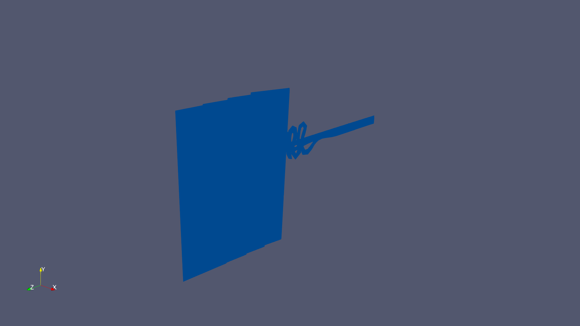
📝 points-surf-clip

40/55 (72.7%)

📋 Task Description

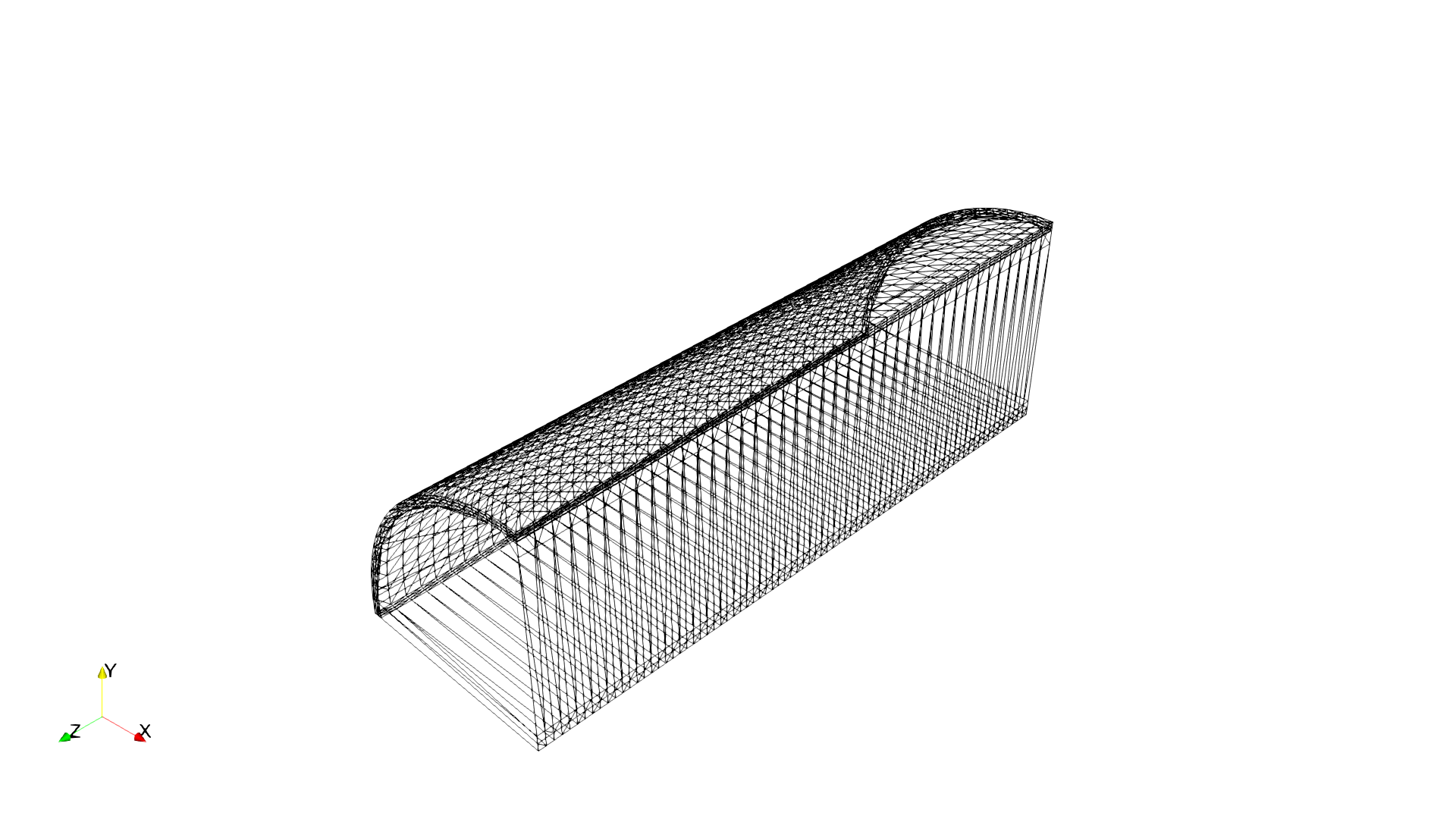
I would like to use ParaView to visualize a dataset. Read in the file named "points-surf-clip/data/points-surf-clip.ex2". Generate an 3d Delaunay triangulation of the dataset. Clip the data with a y-z plane at x=0, keeping the -x half of the data and removing the +x half. Render the image as a wireframe. Save a screenshot of the result in the filename "points-surf-clip/results/{agent_mode}/points-surf-clip.png". The rendered view and saved screenshot should be 1920 x 1080 pixels. Use a white background color. (Optional, but must save if use paraview) Save the paraview state as "points-surf-clip/results/{agent_mode}/points-surf-clip.pvsm". (Optional, but must save if use python script) Save the python script as "points-surf-clip/results/{agent_mode}/points-surf-clip.py". Do not save any other files, and always save the visualization image.

🖼️ Visualization Comparison

Ground Truth

Agent Result

📏 Vision Evaluation Rubrics

Score Summary

Total Score

27/40

Goals

4

Points/Goal

10

Goal 1

8/10

Criterion: Delaunay Triangulation Quality: Is the 3D Delaunay triangulation properly generated creating a valid mesh structure from the point data?

Judge's Assessment: The result shows a dense, connected triangulated/wireframe mesh consistent with a 3D Delaunay tetrahedralization (interior diagonals and surface triangulation are visible). Compared to the ground truth, the mesh structure looks broadly similar, though the result appears visually heavier/overdrawn in places (likely due to viewpoint/edge overlap), making it harder to verify the same triangulation density and distribution.

Goal 2

5/10

Criterion: Clipping Accuracy: Is the mesh correctly clipped by the y-z plane at x=0, with only the -x half of the data remaining visible?

Judge's Assessment: The clipping plane effect is present (a cut face is visible), but the remaining portion does not match the ground truth’s clipped half-cylinder/elongated shape. The result looks like a quarter/side section presented from a different orientation and possibly clipped differently (or with an additional/incorrect clip), so it’s not clearly showing the “keep -x, remove +x” half as in the reference.

Goal 3

8/10

Criterion: Wireframe Representation: Is the result displayed as a clear wireframe showing the triangulated mesh structure with visible edges?

Judge's Assessment: Wireframe rendering is clearly used: edges are visible and the mesh is drawn with black lines on a white background, consistent with the requirement. However, the result has substantial line overplotting (thick dark regions), reducing clarity compared with the ground truth’s cleaner wireframe appearance.

Goal 4

6/10

Criterion: Geometric Integrity: Does the clipped wireframe maintain proper connectivity and show the expected geometric features without artifacts?

Judge's Assessment: Connectivity is mostly intact and the clipped boundary is coherent, but there are noticeable artifacts from overdraw/aliasing and the geometry presentation differs from the ground truth (the expected long clipped volume is not shown). This makes the geometric features less interpretable and suggests a mismatch in camera/clipping configuration.

Overall Assessment

The output correctly produces a triangulated wireframe on a white background, but it does not match the ground truth’s clipped half-volume view. The biggest discrepancy is clipping/camera configuration: the result shows a different remaining section/appearance than the expected -x half after clipping at x=0, and the wireframe is visually cluttered compared to the reference.

📊 Detailed Metrics

Visualization Quality

27/40

Output Generation

5/5

Efficiency

8/10

Completed in 98.70 seconds (good)

📝 render-histogram

42/55 (76.4%)

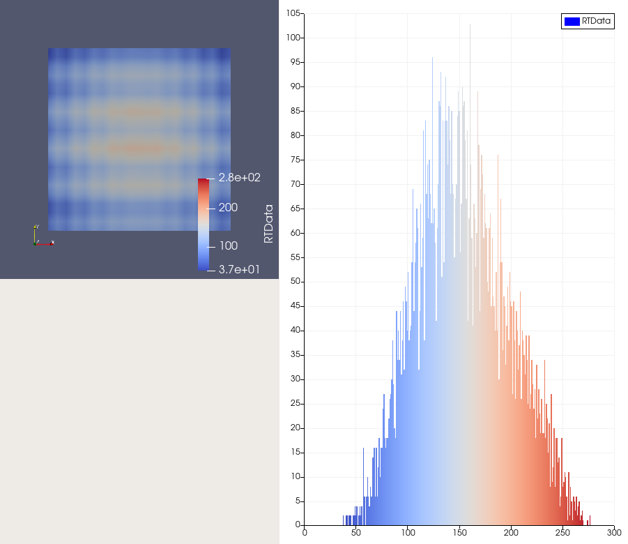
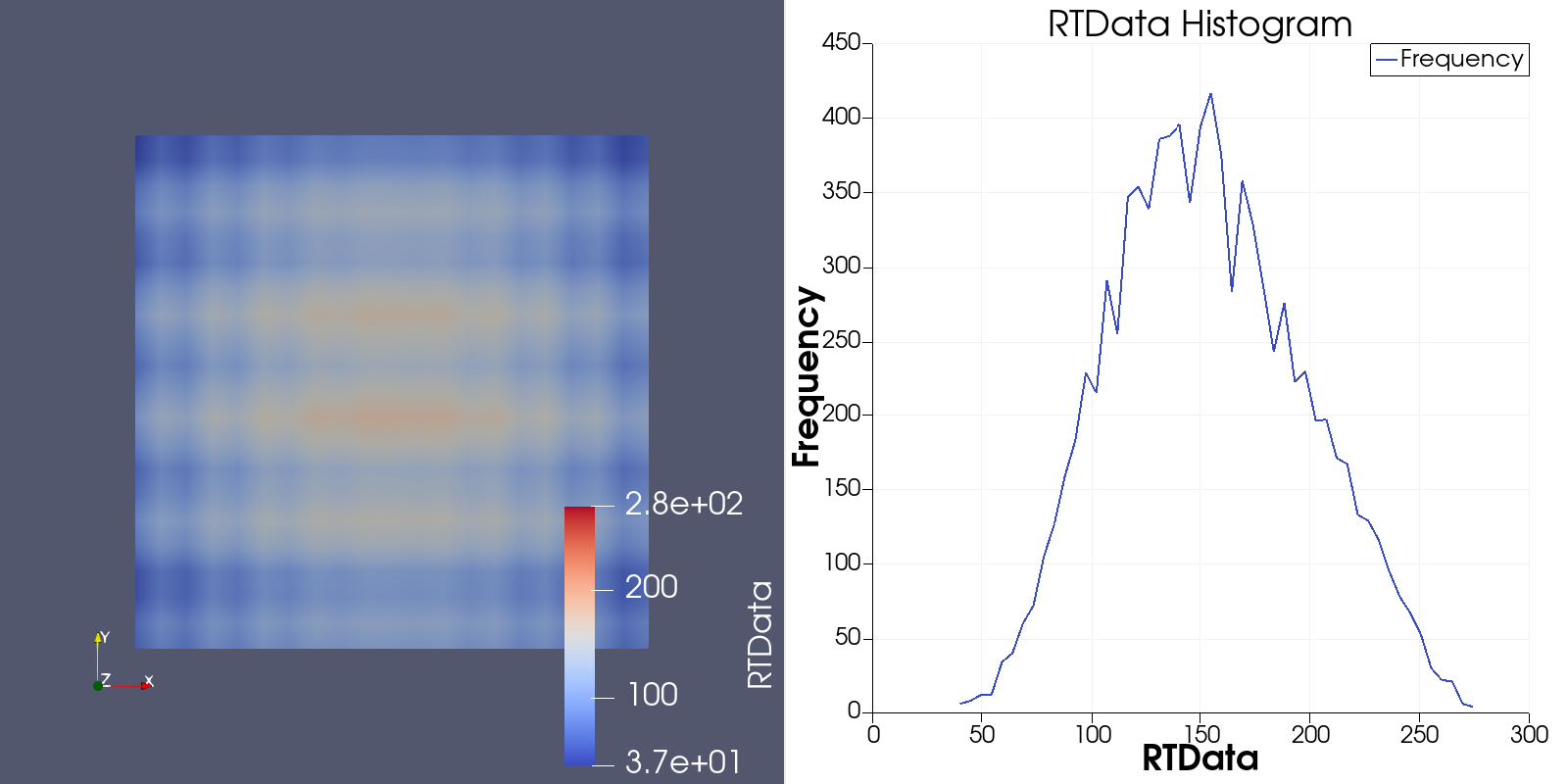
📋 Task Description

Create a wavelet object and render it as a surface colored by RTDATA with a visible color bar. Rescale the colors to the data range and use the 'Cool to Warm' color map. Next, split the view horizontally to the right and create a histogram view from the wavelet RTDATA. Apply the same 'Cool to Warm' color map to the histogram. Save a screenshot of both views (wavelet rendering on the left and histogram on the right) in the file "render-histogram/results/{agent_mode}/render-histogram.png". (Optional, but must save if use paraview) Save the paraview state as "render-histogram/results/{agent_mode}/render-histogram.pvsm". (Optional, but must save if use python script) Save the python script as "render-histogram/results/{agent_mode}/render-histogram.py". Do not save any other files, and always save the visualization image.

🖼️ Visualization Comparison

Ground Truth

Agent Result

📏 Vision Evaluation Rubrics

Score Summary

Total Score

29/40

Goals

4

Points/Goal

10

Goal 1

9/10

Criterion: Wavelet Visualization: Is the wavelet object properly rendered with RTDATA coloring and visible color bar?

Judge's Assessment: Result wavelet rendering (left) matches the ground truth: a wavelet surface colored by RTData with a visible cool-to-warm color bar. Color bar range/labels (approx 3.7e+01 to 2.8e+02) and general appearance align closely; only minor differences in zoom/camera framing.

Goal 2

10/10

Criterion: Split View Layout: Is the view correctly split with the wavelet visualization on the left and histogram on the right?

Judge's Assessment: Layout matches perfectly: horizontally split view with the wavelet rendering on the left and the histogram view on the right, similar proportions to the ground truth.

Goal 3

6/10

Criterion: Histogram Generation: Is the histogram properly generated from RTDATA showing the data distribution?

Judge's Assessment: A histogram-like distribution is shown on the right, but it does not match the ground truth histogram rendering: the ground truth shows vertical colored bars (binned histogram), while the result shows a single blue line curve labeled Frequency vs RTData, which looks like a line plot of bin counts rather than a bar histogram.

Goal 4

4/10

Criterion: Color Map Consistency: Are both the wavelet visualization and histogram using the same Cool to Warm color map?

Judge's Assessment: Colormap consistency is not met: the wavelet uses a cool-to-warm map, but the histogram in the result is monochrome blue (line) rather than using the same cool-to-warm coloring across bins as in the ground truth.

Overall Assessment

The wavelet rendering and split-screen layout closely match the ground truth, including a visible cool-to-warm color bar on the wavelet. However, the histogram view differs substantially: it is rendered as a single blue line (and not cool-to-warm colored bars), so the histogram generation style and colormap consistency requirements are only partially satisfied.

📊 Detailed Metrics

Visualization Quality

29/40

Output Generation

5/5

Efficiency

8/10

Completed in 102.77 seconds (good)

📝 reset-camera-direction

52/55 (94.5%)

📋 Task Description

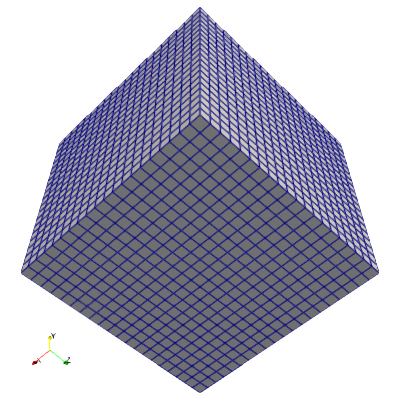
Create a Wavelet object, set its representation to "Surface with Edges", and set the camera direction to [0.5, 1, 0.5]. Save a screenshot to the file "reset-camera-direction/results/{agent_mode}/reset-camera-direction.png". (Optional, but must save if use paraview) Save the paraview state as "reset-camera-direction/results/{agent_mode}/reset-camera-direction.pvsm". (Optional, but must save if use python script) Save the python script as "reset-camera-direction/results/{agent_mode}/reset-camera-direction.py". Do not save any other files, and always save the visualization image.

🖼️ Visualization Comparison

Ground Truth

Agent Result

📏 Vision Evaluation Rubrics

Score Summary

Total Score

37/40

Goals

4

Points/Goal

10

Goal 1

10/10

Criterion: Wavelet Creation: Is the Wavelet object properly created and displayed in the scene?

Judge's Assessment: The result image shows the expected Wavelet source rendered as a cube-like volume, matching the ground truth geometry and presence in the scene.

Goal 2

10/10

Criterion: Surface with Edges Representation: Is the wavelet correctly displayed with "Surface with Edges" representation showing both surface and wireframe?

Judge's Assessment: Both ground truth and result clearly use "Surface with Edges": shaded faces are visible along with a uniform blue edge grid overlay on the surfaces.

Goal 3

9/10

Criterion: Camera Direction: Is the camera positioned according to the specified direction vector [0.5, 1,

Judge's Assessment: The camera view direction appears to match the ground truth very closely (same three visible faces and similar orientation consistent with direction [0.5, 1, 0.5]). Minor differences are visible in framing/zoom and background styling, but the direction itself looks essentially correct.

Goal 4

8/10

Criterion: 5]?

Judge's Assessment: The wavelet is clearly visible and well-oriented, but the result differs from the ground truth in view presentation (darker background, slightly different zoom/cropping and no white margin), which modestly affects visual comparability though not clarity.

Overall Assessment

The result successfully creates and displays the Wavelet with the correct "Surface with Edges" representation and a camera orientation that closely matches the specified direction. Differences are mainly aesthetic/framing rather than substantive.

📊 Detailed Metrics

Visualization Quality

37/40

Output Generation

5/5

Efficiency

10/10

Completed in 28.43 seconds (excellent)

📝 richtmyer

33/45 (73.3%)

📋 Task Description

Task: Load the Richtmyer dataset from "richtmyer/data/richtmyer_256x256x240_float32.vtk". Generate a visualization image of the Richtmyer dataset, Entropy field (timestep 160) of Richtmyer-Meshkov instability simulation, with the following visualization settings: 1) Create volume rendering 2) Set the opacity transfer function as a ramp function from value 0.05 to 1 of the volumetric data, assigning opacity 0 to value less than 0.05 and assigning opacity 1 to value 1. 3) Set the color transfer function following the 7 rainbow colors and assign a red color [1.0, 0.0, 0.0] to the highest value, a purple color [0.5, 0.0, 1.0] to the lowest value. 4) Visualization image resolution is 1024x1024 5) Set the viewpoint parameters as: [420, 420, -550] to position; [128, 128, 150] to focal point; [-1, -1, 1] to camera up direction 6) Turn on the shade and set the ambient, diffuse and specular as 1.0 7) White background. Volume rendering ray casting sample distance is 0.1 8) Don't show color/scalar bar or coordinate axes. Save the visualization image as "richtmyer/results/{agent_mode}/richtmyer.png". (Optional, but must save if use paraview) Save the paraview state as "richtmyer/results/{agent_mode}/richtmyer.pvsm". (Optional, but must save if use pvpython script) Save the python script as "richtmyer/results/{agent_mode}/richtmyer.py". (Optional, but must save if use VTK) Save the cxx code script as "richtmyer/results/{agent_mode}/richtmyer.cxx" Do not save any other files, and always save the visualization image.

🖼️ Visualization Comparison

Ground Truth

Agent Result

📏 Vision Evaluation Rubrics

Score Summary

Total Score

20/30

Goals

3

Points/Goal

10

Goal 1

8/10

Criterion: Does the visualization show a clear surface with peaks and valleys?

Judge's Assessment: Both ground truth and result show a clearly defined volumetric surface with strong textured structure (many bubble-like peaks and valleys) and the same overall pyramid/diamond silhouette. The result is slightly darker overall and has less visible warm-color detail on the top surface compared with the ground truth, but the surface relief is still clear.

Goal 2

4/10

Criterion: Are the peaks highlighted with the reddish color?

Judge's Assessment: In the ground truth, many local high-value features on the surface are highlighted with yellow/orange to red accents, and the side faces are strongly red. In the result, the top surface is dominated by blues/teals with very limited red/orange highlighting; the most intense reds are largely absent on the surface (and the side faces appear dark/blackish with red striping rather than solid red). This indicates high-value (peak) coloring does not match well.

Goal 3

8/10

Criterion: Are the valleys highlighted with the bluish color?

Judge's Assessment: Valley/low regions are predominantly bluish in both images, especially across the top surface where depressions and background texture are blue/teal. The result is even more strongly blue overall than the ground truth, but it still satisfies the valley-low-to-blue mapping well.

Overall Assessment

The geometry/structure of the volume rendering matches the ground truth well (clear peaks and valleys), and low-value regions are correctly emphasized with blues. However, the result substantially under-represents the warm/red colors associated with high values on the main surface, making peak highlighting notably worse than in the ground truth.

📊 Detailed Metrics

Visualization Quality

20/30

Output Generation

5/5

Efficiency

8/10

Completed in 111.97 seconds (good)

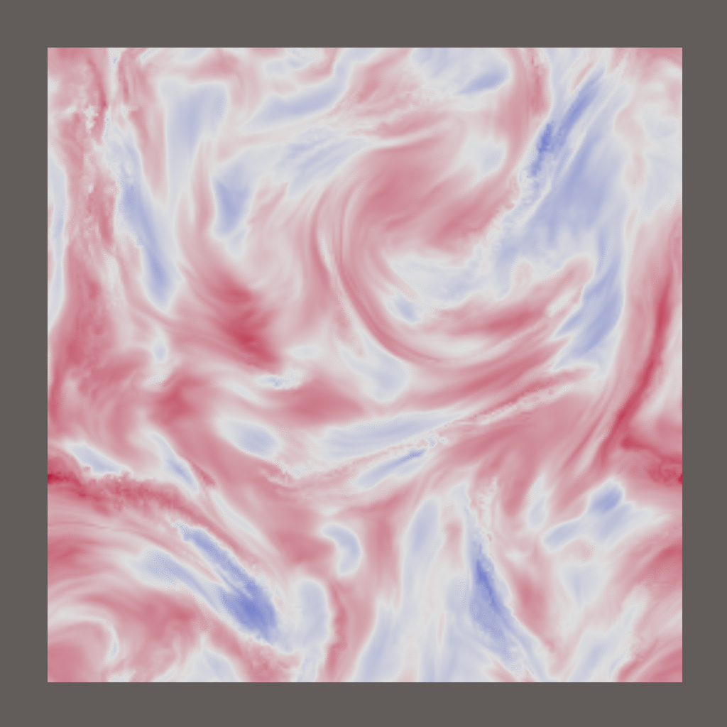
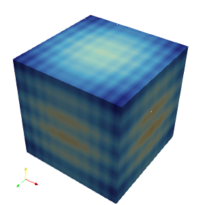
📝 rotstrat

30/45 (66.7%)

📋 Task Description

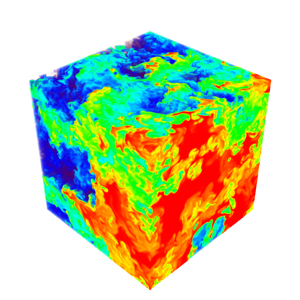
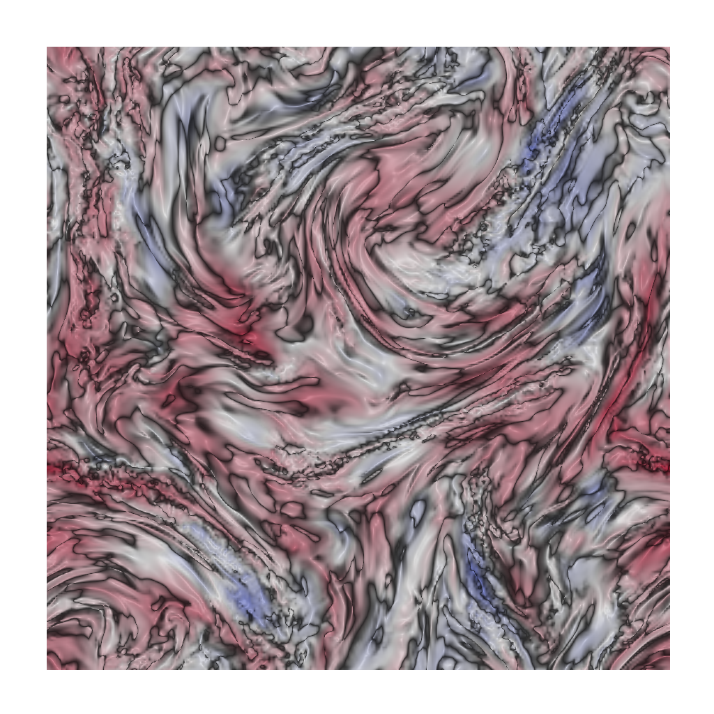
Task: Load the rotstrat dataset from "rotstrat/data/rotstrat_256x256x256_float32.vtk". Generate a visualization image of the Rotstrat dataset, temperature field of a direct numerical simulation of rotating stratified turbulence, with the following visualization settings: 1) Create volume rendering 2) Set the opacity transfer function as a step function jumping from 0 to 1 at value 0.12 3) Set the color transfer function to assign a warm red color [0.71, 0.02, 0.15] to the highest value, a cool color [0.23, 0.29, 0.75] to the lowest value, and a grey color[0.87, 0.87, 0.87] to the midrange value 4) Set the viewpoint parameters as: [800, 128, 128] to position; [0, 128, 128] to focal point; [0, 1, 0] to camera up direction 5) Volume rendering ray casting sample distance is 0.1 6) White background 7) Visualization image resolution is 1024x1024 8) Don't show color/scalar bar or coordinate axes. Save the visualization image as "rotstrat/results/{agent_mode}/rotstrat.png". (Optional, but must save if use paraview) Save the paraview state as "rotstrat/results/{agent_mode}/rotstrat.pvsm". (Optional, but must save if use pvpython script) Save the python script as "rotstrat/results/{agent_mode}/rotstrat.py". (Optional, but must save if use VTK) Save the cxx code script as "rotstrat/results/{agent_mode}/rotstrat.cxx" Do not save any other files, and always save the visualization image.

🖼️ Visualization Comparison

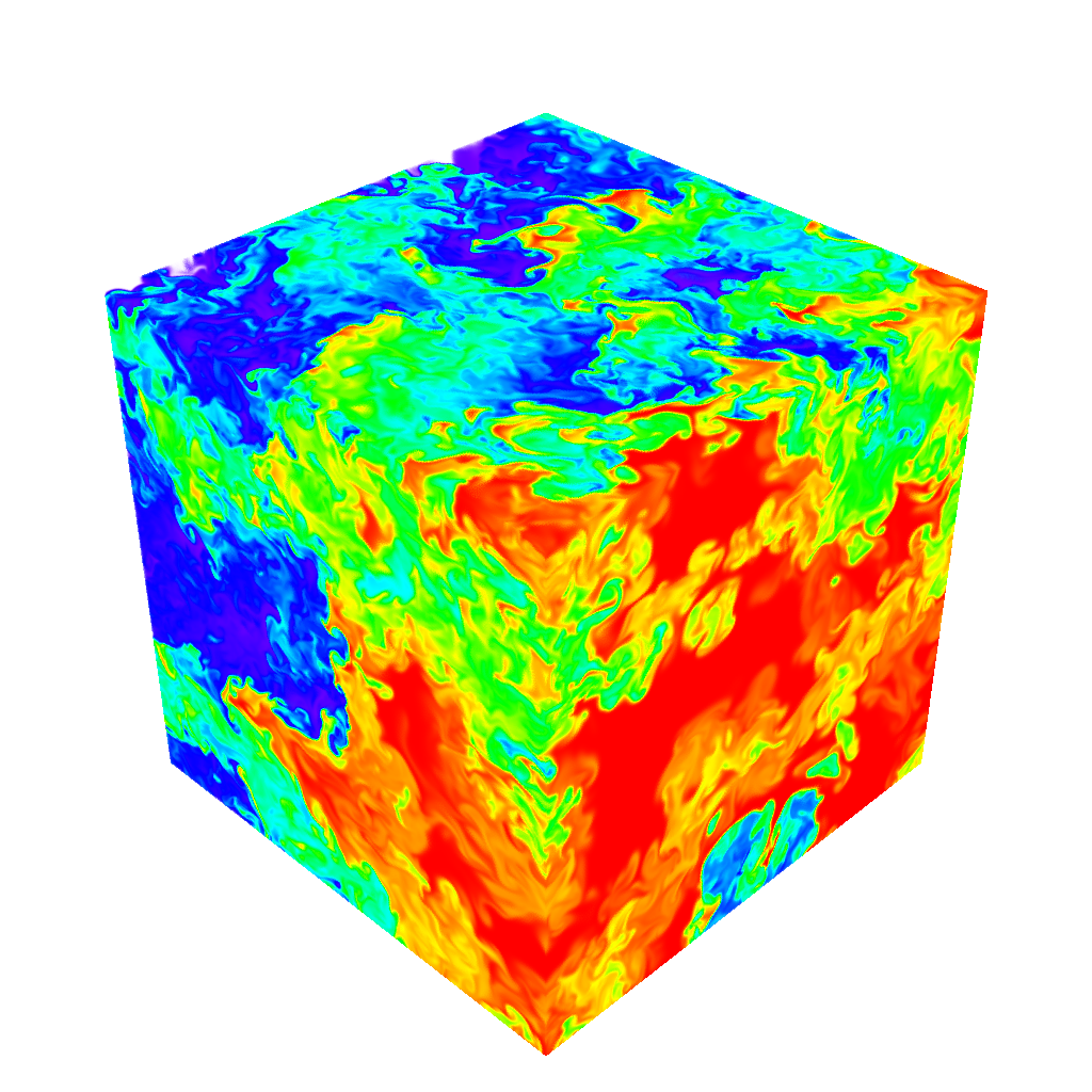
Ground Truth

Agent Result

📏 Vision Evaluation Rubrics

Score Summary

Total Score

16/30

Goals

3

Points/Goal

10

Goal 1

5/10

Criterion: Does the visualization image clearly show the shape of turbulence compared to ground truth?

Judge's Assessment: The ground truth shows sharp, high-contrast turbulent filamentary structures with pronounced grey midtones and dark boundary-like contours, giving a detailed ‘textured’ turbulence appearance. The result image has a much softer, blurred look with significantly reduced fine-scale structure and contrast; the overall turbulent pattern is present but lacks the crispness and opacity/step-function-driven delineation seen in the ground truth. Also, the result has a dark gray surrounding frame rather than the clean white background/margins of the ground truth composition.

Goal 2

6/10

Criterion: Does the visualization show the shape of a vortex in the upper right part of the image?

Judge's Assessment: In the ground truth, the upper-right region contains a clearly defined vortex/roll structure with tight curvature and visible internal filament detail. In the result, a similarly located swirling feature exists, but it is much more diffuse and the vortex boundary is not as clearly separated from the surrounding flow, making the vortex shape only moderately comparable.

Goal 3

5/10

Criterion: Does the visualization show the shape of a vortex in the bottom left corner of the image?

Judge's Assessment: The ground truth bottom-left corner shows a distinct curled vortex-like structure with clear layered/striated detail. The result bottom-left has a broadly similar curved flow feature, but it is washed out and less localized; the vortex in that corner is not as clearly identifiable or sharply formed as in the ground truth.

Overall Assessment

The result captures the general large-scale swirl/turbulence layout and includes vortex-like features in the indicated regions, but it deviates notably from the ground truth in sharpness, opacity/contrast (step-function effect), and fine structural detail, leading to only partial matches for turbulence and the two vortex-shape criteria.

📊 Detailed Metrics

Visualization Quality

16/30

Output Generation

5/5

Efficiency

9/10

Completed in 64.49 seconds (very good)

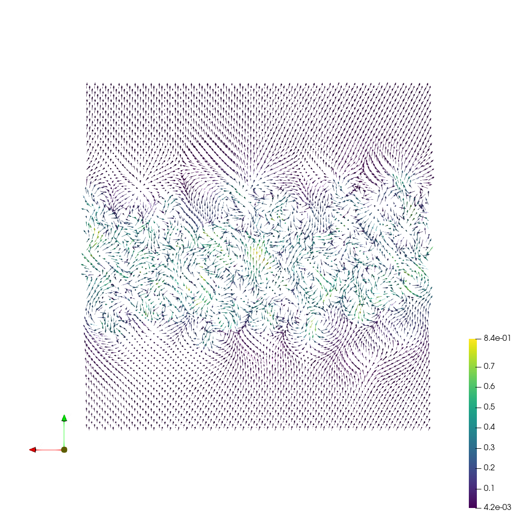
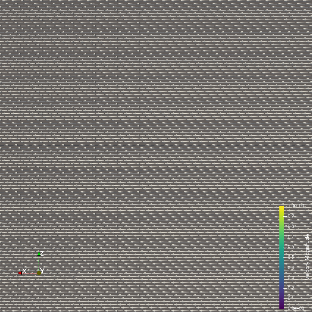
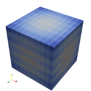
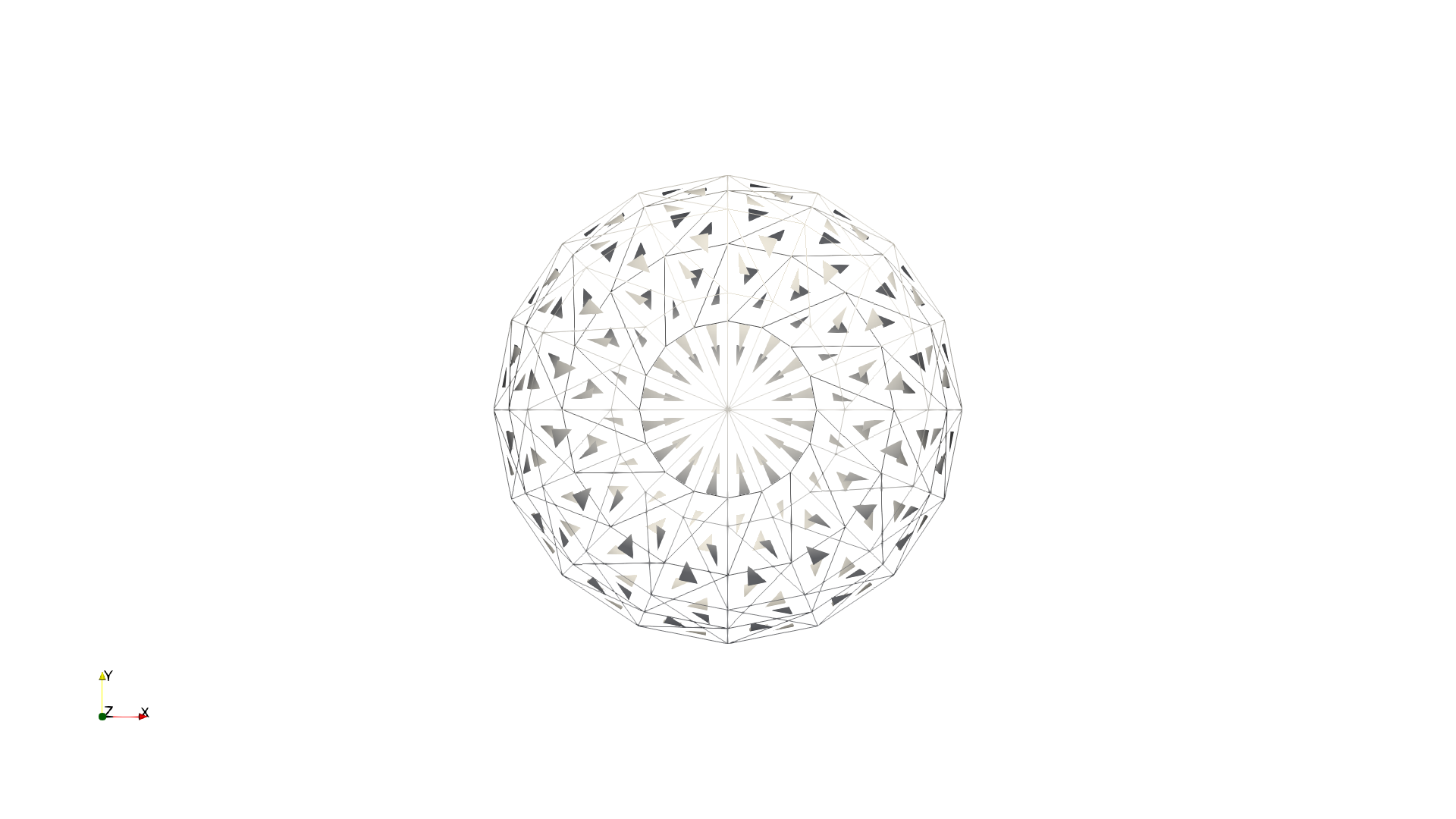
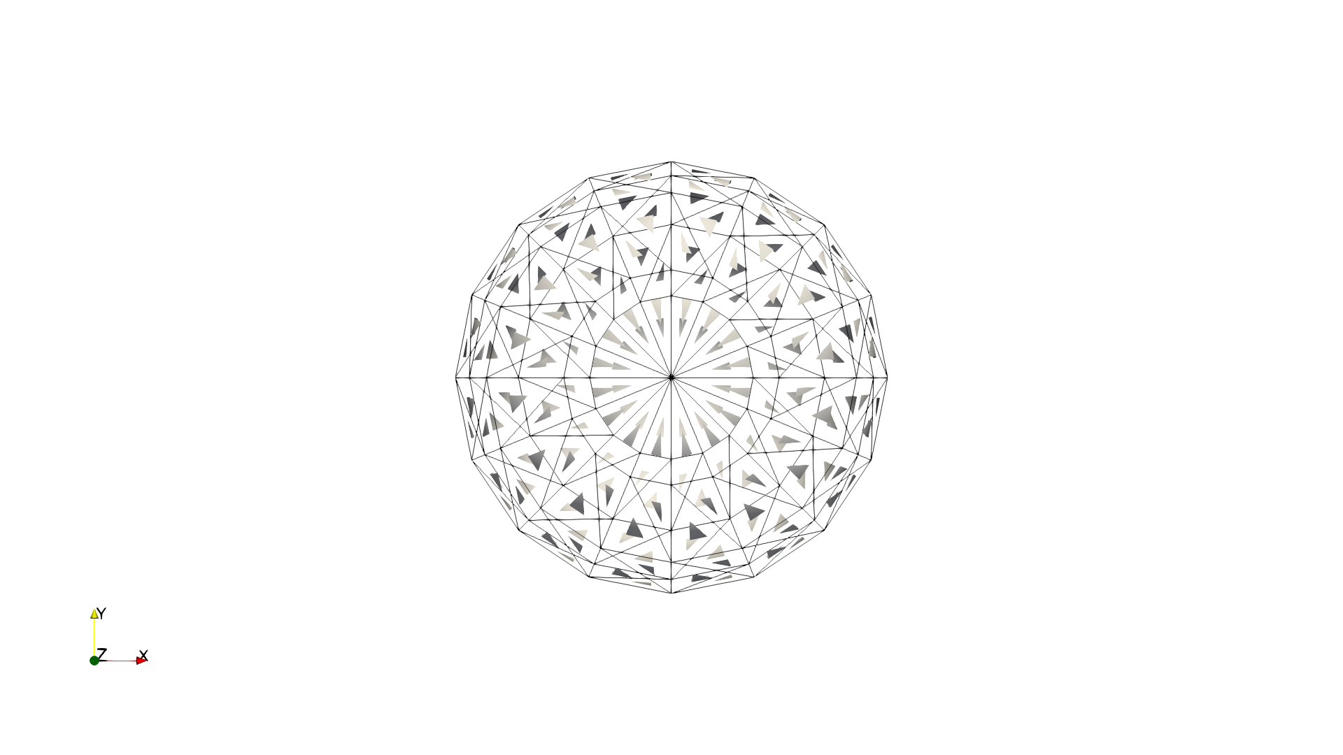
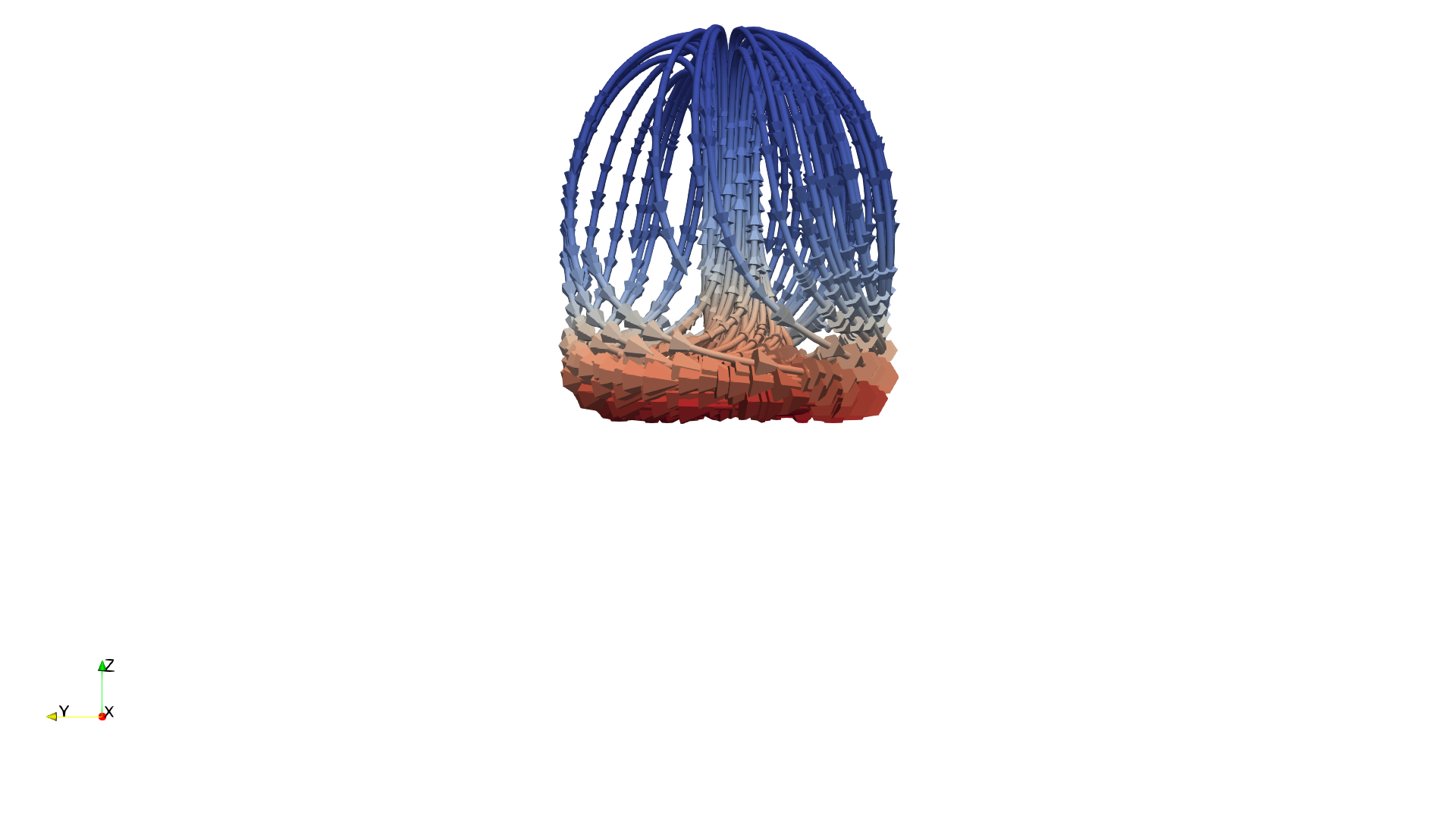
📝 rti-velocity_glyph

⚠️ LOW SCORE

27/55 (49.1%)

📋 Task Description

Load the Rayleigh-Taylor instability velocity field dataset from "rti-velocity_glyph/data/rti-velocity_glyph.vti" (VTI format, 128x128x128 grid). Create a slice at y=64 through the volume. Place arrow glyphs on the slice, oriented by the velocity vector. Use uniform arrow size (no magnitude scaling, scale factor 3.0). Color the arrows by velocity magnitude using the 'Viridis (matplotlib)' colormap. Use a sampling stride of 3. Add a color bar labeled 'Velocity Magnitude'. Use a white background. Set the camera to view along the negative y-axis. Render at 1024x1024. Set the viewpoint parameters as: [63.5, 250.0, 63.5] to position; [63.5, 64.0, 63.5] to focal point; [0.0, 0.0, 1.0] to camera up direction. Save the visualization image as "rti-velocity_glyph/results/{agent_mode}/rti-velocity_glyph.png". (Optional, but must save if use paraview) Save the paraview state as "rti-velocity_glyph/results/{agent_mode}/rti-velocity_glyph.pvsm". (Optional, but must save if use pvpython script) Save the python script as "rti-velocity_glyph/results/{agent_mode}/rti-velocity_glyph.py". (Optional, but must save if use VTK) Save the cxx code script as "rti-velocity_glyph/results/{agent_mode}/rti-velocity_glyph.cxx" Do not save any other files, and always save the visualization image.

🖼️ Visualization Comparison

Ground Truth

Agent Result

📏 Vision Evaluation Rubrics

Score Summary

Total Score

14/40

Goals

4

Points/Goal

10

Goal 1

3/10

Criterion: Overall Visualization Goal: Does the result match the ground truth glyph visualization of the RTI velocity field?

Judge's Assessment: Ground truth shows a y=64 slice with a prominent turbulent/roll-up band across the middle and calmer regions above/below, rendered on a white background with a Viridis-colored magnitude colorbar. The result image instead shows a nearly uniform field of arrows across the entire slice with a dark gray background and no visible RTI roll-up structure, so the overall visualization goal is largely not achieved.

Goal 2

2/10

Criterion: Glyph Patterns: Do the arrow glyphs show similar orientation and spatial patterns as the ground truth?

Judge's Assessment: In the ground truth, glyph directions vary strongly, forming vortical/curled patterns concentrated in the central mixing layer and more coherent flow above and below. In the result, arrows are almost all aligned in the same direction (predominantly horizontal) with minimal directional variation, failing to reproduce the spatial orientation patterns.

Goal 3

6/10

Criterion: Glyph Appearance: Do the glyphs appear with similar uniform sizing as the ground truth?

Judge's Assessment: Both images use uniformly sized arrows (no obvious magnitude-based scaling). However, the result appears much denser and more visually uniform (suggesting a different sampling/stride and/or glyph scaling relative to the view), so while uniform sizing is mostly satisfied, it does not match the ground-truth appearance closely.

Goal 4

3/10

Criterion: Color Mapping: Is the color distribution across glyphs visually similar to the ground truth?

Judge's Assessment: Ground truth uses Viridis with clear variation (purple/blue in low-speed regions and green/yellow highlights in the central band). The result’s arrows appear mostly gray/white with little visible Viridis variation across the field; although a Viridis-like colorbar is present, the mapped colors on glyphs do not resemble the ground truth distribution.

Overall Assessment

The result diverges substantially from the expected RTI slice glyph visualization: the flow structure/orientation patterns are missing, the background is not white, and color-by-magnitude variation is not visually expressed on the glyphs. The only partially matching aspect is the use of uniform glyph sizing and inclusion of a Viridis-style colorbar.

📊 Detailed Metrics

Visualization Quality

14/40

Output Generation

5/5

Efficiency

8/10

Completed in 110.15 seconds (good)

PSNR

19.16 dB

SSIM

0.9233

LPIPS

0.0816

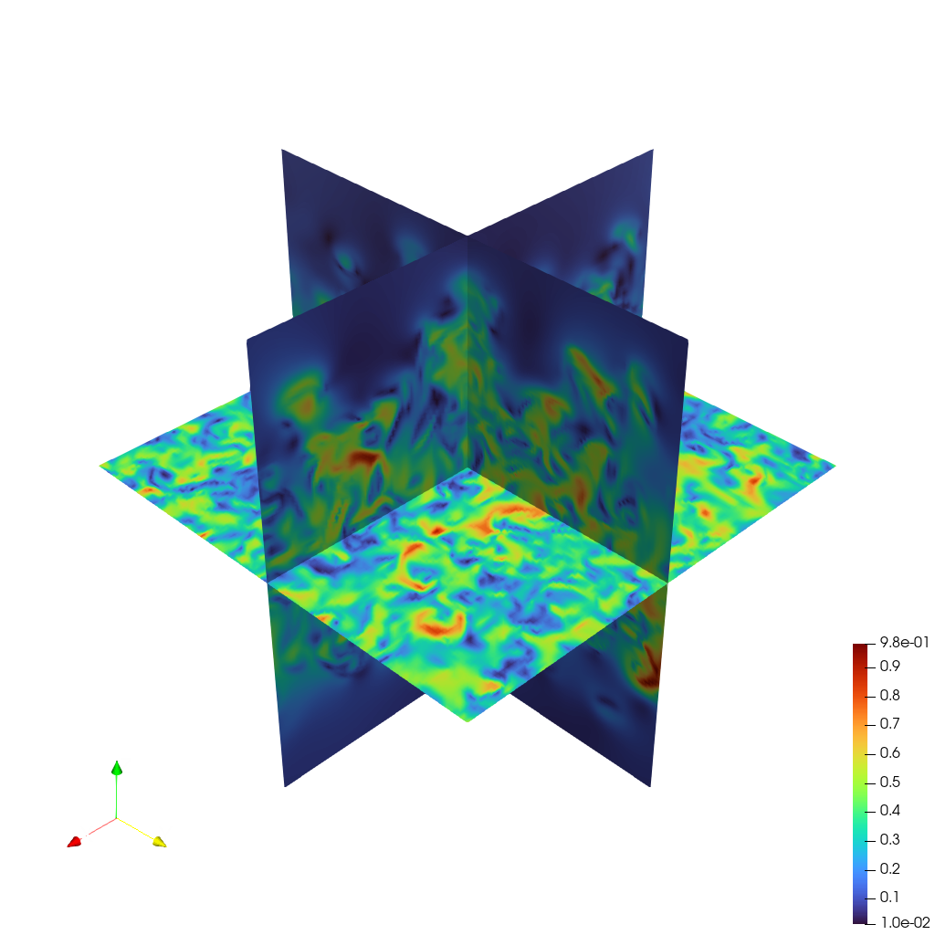
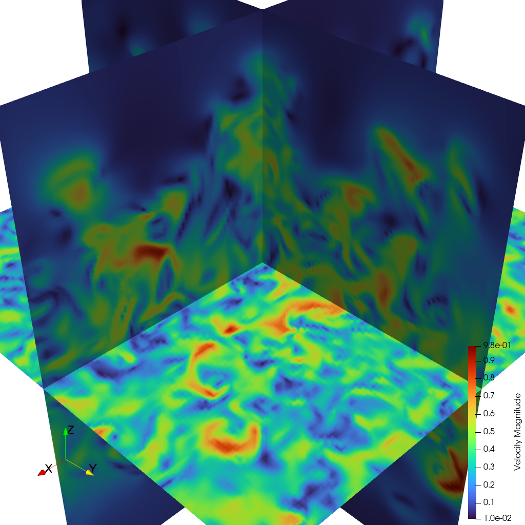
📝 rti-velocity_slices

40/45 (88.9%)

📋 Task Description

Load the Rayleigh-Taylor instability velocity field from "rti-velocity_slices/data/rti-velocity_slices.vti" (VTI format, 128x128x128). Create three orthogonal slices: at x=64 (YZ-plane), y=64 (XZ-plane), and z=64 (XY-plane). Color all three slices by velocity magnitude using the 'Turbo' colormap. Add a color bar labeled 'Velocity Magnitude'. Use a white background. Set an isometric camera view that shows all three slices. Render at 1024x1024. Set the viewpoint parameters as: [200.0, 200.0, 200.0] to position; [63.5, 63.5, 63.5] to focal point; [0.0, 0.0, 1.0] to camera up direction. Save the visualization image as "rti-velocity_slices/results/{agent_mode}/rti-velocity_slices.png". (Optional, but must save if use paraview) Save the paraview state as "rti-velocity_slices/results/{agent_mode}/rti-velocity_slices.pvsm". (Optional, but must save if use pvpython script) Save the python script as "rti-velocity_slices/results/{agent_mode}/rti-velocity_slices.py". (Optional, but must save if use VTK) Save the cxx code script as "rti-velocity_slices/results/{agent_mode}/rti-velocity_slices.cxx" Do not save any other files, and always save the visualization image.

🖼️ Visualization Comparison

Ground Truth

Agent Result

📏 Vision Evaluation Rubrics

Score Summary

Total Score

28/30

Goals

3

Points/Goal

10

Goal 1

10/10

Criterion: Slice Count and Orientation: Are there exactly three perpendicular slices (one horizontal XY-plane and two vertical XZ and YZ planes), matching the ground truth arrangement?

Judge's Assessment: The result shows exactly three mutually orthogonal slices intersecting at the volume center: one horizontal XY slice and two vertical slices (XZ and YZ). Their spatial arrangement and isometric view match the ground truth (same cross-like configuration with all three planes visible).

Goal 2

9/10

Criterion: Color Mapping: Are the slices colored using a Turbo-like colormap (blue to green to yellow to red) mapped to velocity magnitude, with a similar color distribution as the ground truth?

Judge's Assessment: The slices are colored with a Turbo-like rainbow (dark blue/purple through cyan/green to yellow/red), consistent with velocity magnitude coloring in the ground truth. The overall color distribution is very similar; minor differences may exist in contrast/opacity or exact range mapping, but the colormap intent is clearly correct. A colorbar labeled 'Velocity Magnitude' is present as expected.

Goal 3

9/10

Criterion: Mixing Zone Pattern: Does the horizontal (XY) slice show a chaotic, high-velocity-magnitude mixing pattern in its center region, similar to the ground truth?

Judge's Assessment: The horizontal (XY) slice exhibits the expected chaotic mixing-zone texture with mottled, swirling structures and scattered high-magnitude hotspots (yellow/red) concentrated through the interior, matching the ground truth pattern closely. Any differences are minor (slightly different prominence of hotspots due to scaling/opacity).

Overall Assessment

Overall, the result matches the ground truth very well: correct three-slice orthogonal setup, appropriate Turbo-style magnitude coloring with labeled colorbar, and a convincingly similar RTI mixing pattern on the central XY slice. Only small, non-critical differences in color scaling/contrast are noticeable.

📊 Detailed Metrics

Visualization Quality

28/30

Output Generation

5/5

Efficiency

7/10

Completed in 186.47 seconds (acceptable)

PSNR

19.27 dB

SSIM

0.9609

LPIPS

0.0414

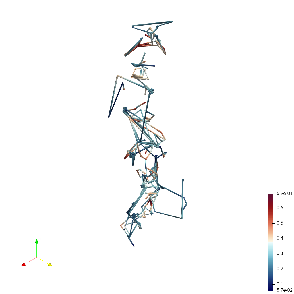
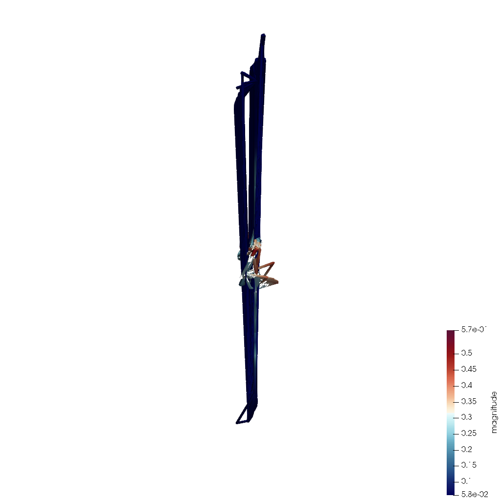
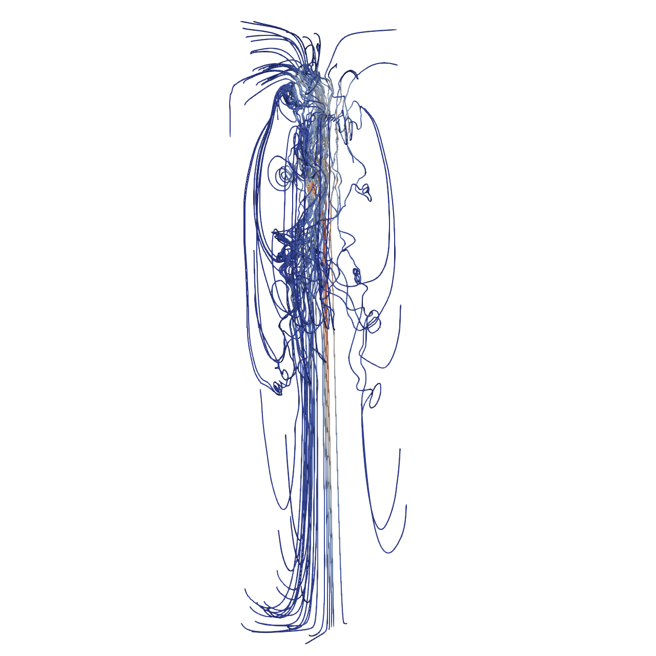
📝 rti-velocity_streakline

23/45 (51.1%)

📋 Task Description

Load the Rayleigh–Taylor instability velocity field time series from "rti-velocity_streakline/data/rti-velocity_streakline_{timestep}.nc", where "timestep" in {0030, 0031, 0032, 0033, 0034, 0035, 0036, 0037, 0038, 0039, 0040} (11 timesteps, NetCDF format, 128×128×128 grid each, with separate vx, vy, vz arrays). Construct the time-varying velocity field u(x,t) by merging vx, vy, vz into a single vector field named "velocity", and compute the velocity magnitude "magnitude" = |velocity| for coloring. Compute streaklines as a discrete approximation of continuous particle injection: continuously release particles from fixed seed points at every sub-timestep into the time-varying velocity field using the StreakLine filter. Apply TemporalShiftScale (scale=20) to extend particle travel time, and apply TemporalInterpolator with a sub-timestep interval of 0.25 (or smaller) to approximate continuous injection over time. Seed 26 static points along a line on the z-axis at x=64, y=64 (from z=20 to z=108). Use StaticSeeds=True, ForceReinjectionEveryNSteps=1 (reinjection at every sub-timestep), and set TerminationTime=200. Render the resulting streaklines as tubes with radius 0.3. Color the tubes by velocity magnitude ("magnitude") using the 'Cool to Warm (Extended)' colormap. Add a color bar for velocity magnitude. Use a white background. Set an isometric camera view and render at 1024×1024. Set the viewpoint parameters as: [200.0, 200.0, 200.0] to position; [63.5, 63.5, 63.5] to focal point; [0.0, 0.0, 1.0] to camera up direction. Save the visualization image as "rti-velocity_streakline/results/{agent_mode}/rti-velocity_streakline.png". (Optional, but must save if use paraview) Save the paraview state as "rti-velocity_streakline/results/{agent_mode}/rti-velocity_streakline.pvsm". (Optional, but must save if use pvpython script) Save the python script as "rti-velocity_streakline/results/{agent_mode}/rti-velocity_streakline.py". (Optional, but must save if use VTK) Save the cxx code script as "rti-velocity_streakline/results/{agent_mode}/rti-velocity_streakline.cxx" Do not save any other files, and always save the visualization image.

🖼️ Visualization Comparison

Ground Truth

Agent Result

📏 Vision Evaluation Rubrics

Score Summary

Total Score

9/30

Goals

3

Points/Goal

10

Goal 1

3/10

Criterion: Streak Line Patterns: Do the streak lines show similar flow patterns and structures as the ground truth?

Judge's Assessment: Ground truth shows many kinked/looping streakline segments forming a tangled, branching structure across a moderate vertical span, with multiple turns and lateral excursions. The result image instead is dominated by a few nearly straight, very long vertical tubes (dark blue) with only a small cluster of tangled lines near the center. The core streakline pattern/structure (many short, angular, crisscrossing trajectories) is largely missing or overwhelmed by the vertical features.

Goal 2

2/10

Criterion: Streak Line Coverage: Is the spatial extent and distribution of streak lines similar to the ground truth?

Judge's Assessment: Ground truth has streaklines distributed throughout a larger 3D region around the seed line, producing broad coverage and many distinct trajectories. The result has extremely limited spatial distribution: most geometry collapses into a narrow column with a couple of long vertical paths and minimal lateral spread, so the extent and distribution do not match the ground truth.

Goal 3

4/10

Criterion: Color Mapping: Is the color distribution along streak lines visually similar to the ground truth?

Judge's Assessment: Both use a cool-to-warm style map and show some warm colors at higher magnitudes, but the ground truth exhibits varied coloring along many streakline segments (balanced mix of blues/cyans with intermittent whites/oranges/reds). The result is predominantly dark blue along the long vertical tubes with only a small warm-colored region near the center, indicating a substantially different magnitude distribution (and possibly different scalar range/normalization).

Overall Assessment

The result deviates strongly from the ground truth: streakline geometry is dominated by a few long vertical tubes with minimal spread, whereas the ground truth shows a complex, tangled set of streaklines with broader coverage and more varied color distribution. Colormap choice is roughly consistent, but the mapped magnitude appearance and spatial/structural streakline behavior do not match.

📊 Detailed Metrics

Visualization Quality

9/30

Output Generation

5/5

Efficiency

9/10

Completed in 70.70 seconds (very good)

PSNR

17.12 dB

SSIM

0.9337

LPIPS

0.1042

📝 save-transparent

34/35 (97.1%)

📋 Task Description

I would like to use ParaView to visualize a dataset. Create a wavelet object and show it. Color the rendering by the variable ‘RTData’. Render the wavelet as a surface. Hide the color bar. Next, set the layout size to be 300 pixels by 300 pixels. Next, move the camera with the following settings. The camera position should be [30.273897726939246, 40.8733980301544, 43.48927935675712]. The camera view up should be [-0.3634544237682163, 0.7916848767068606, -0.49105594165731975]. The camera parallel scale should be 17.320508075688775. Save a screenshot to the file “save-transparent/results/{agent_mode}/save-transparent.png”, set the image resolution to 300x300, and set the background to transparent. (Optional, but must save if use paraview) Save the paraview state as “save-transparent/results/{agent_mode}/save-transparent.pvsm”. (Optional, but must save if use python script) Save the python script as “save-transparent/results/{agent_mode}/save-transparent.py”. Do not save any other files, and always save the visualization image.

🖼️ Visualization Comparison

Ground Truth

Agent Result

📏 Vision Evaluation Rubrics

Score Summary

Total Score

19/20

Goals

2

Points/Goal

10

Goal 1

9/10

Criterion: Object Creation: Is the wavelet object properly created and displayed in the scene? Looking similar to the GT image?

Judge's Assessment: The result shows the expected wavelet cube rendered as a surface with a similar camera angle and framing to the ground truth. Coloring appears consistent with RTData-style scalar coloring (blue/cyan with some warmer bands). The orientation and overall appearance closely match, with only minor differences in exact colormap intensity/contrast compared to the ground truth.

Goal 2

10/10

Criterion: Transparent Background: Is the screenshot saved with a properly transparent background instead of solid color?

Judge's Assessment: The background is transparent in the result image, matching the ground truth: the cube is rendered over a checkerboard/transparent canvas rather than a solid-color background.

Overall Assessment

Overall the visualization matches the ground truth very well: the wavelet surface is correctly shown with appropriate scalar coloring and the screenshot is saved with a transparent background. Only minor color/contrast differences are visible.

📊 Detailed Metrics

Visualization Quality

19/20

Output Generation

5/5

Efficiency

10/10

Completed in 28.88 seconds (excellent)

📝 shrink-sphere

55/55 (100.0%)

📋 Task Description

Create a default sphere and then hide it. Create a shrink filter from the sphere. Double the sphere's theta resolution. Divide the shrink filter's shrink factor in half. Extract a wireframe from the sphere. Group the shrink filter and wireframe together and show them. Save a screenshot of the result in the filename "shrink-sphere/results/{agent_mode}/shrink-sphere.png". The rendered view and saved screenshot should be 1920 x 1080 pixels and have a white background. (Optional, but must save if use paraview) Save the paraview state as "shrink-sphere/results/{agent_mode}/shrink-sphere.pvsm". (Optional, but must save if use python script) Save the python script as "shrink-sphere/results/{agent_mode}/shrink-sphere.py". Do not save any other files, and always save the visualization image.

🖼️ Visualization Comparison

Ground Truth

Agent Result

📏 Vision Evaluation Rubrics

Score Summary

Total Score

40/40

Goals

4

Points/Goal

10

Goal 1

10/10

Criterion: Sphere Creation and Resolution: Is the sphere created with doubled theta resolution providing higher geometric detail and smoother curvature?

Judge's Assessment: The result sphere shows the same high tessellation/segment density as the ground truth (smooth, many small triangular facets), consistent with a doubled theta resolution. Overall geometry and curvature detail match closely.

Goal 2

10/10

Criterion: Shrink Filter Application: Is the shrink filter properly applied with halved shrink factor creating visible separation between mesh elements?

Judge's Assessment: The shrink effect matches the ground truth: each face appears as a smaller, separated element (dark triangular patches) with the same apparent shrink amount, consistent with halving the shrink factor from the default. The spacing and visual pattern align very well.

Goal 3

10/10

Criterion: Dual Representation: Are both the wireframe sphere and shrink filter results simultaneously visible and properly grouped together?

Judge's Assessment: Both representations are simultaneously visible as in the ground truth: a full wireframe sphere overlay plus the shrunken cell faces inside/offset. The combined appearance indicates the expected grouping/visibility behavior and matches the reference image composition.

Goal 4

10/10

Criterion: Visual Quality: Does the visualization clearly show the contrast between the wireframe structure and the shrunken elements with appropriate white background?

Judge's Assessment: Visual quality matches: white background, clear contrast between thin wireframe lines and darker shrunken facets, and the camera framing/scale are essentially identical to the ground truth. No extra objects or distracting rendering differences are apparent.

Overall Assessment

The result image is an almost exact visual match to the ground truth across geometry resolution, shrink application, dual wireframe+shrink display, and overall rendering quality (white background and clear contrast).

📊 Detailed Metrics

Visualization Quality

40/40

Output Generation

5/5

Efficiency

10/10

Completed in 58.99 seconds (excellent)

📝 solar-plume

46/55 (83.6%)

📋 Task Description

Task: Load the solar plume dataset from "solar-plume/data/solar-plume_126x126x512_float32_scalar3.raw", the information about this dataset: solar-plume (Vector) Data Scalar Type: float Data Byte Order: little Endian Data Extent: 126x126x512 Number of Scalar Components: 3 Data loading is very important, make sure you correctly load the dataset according to their features. Add a "stream tracer" filter under the solar plume data to display streamline, set the "Seed type" to "Point Cloud" and set the center of point cloud to 3D position [50, 50, 320] with a radius 30, then hide the point cloud sphere. Add a "tube" filter under the "stream tracer" filter to enhance the streamline visualization. Set the radius to 0.5. In the pipeline browser panel, hide everything except the "tube" filter. Please think step by step and make sure to fulfill all the visualization goals mentioned above. Set the viewpoint parameters as: [62.51, -984.78, 255.45] to position; [62.51, 62.46, 255.45] to focal point; [0, 0, 1] to camera up direction. Use a white background. Find an optimal view. Render at 1280x1280. Do not show a color bar or coordinate axes. Save the visualization image as "solar-plume/results/{agent_mode}/solar-plume.png". (Optional, but must save if use paraview) Save the paraview state as "solar-plume/results/{agent_mode}/solar-plume.pvsm". (Optional, but must save if use pvpython script) Save the python script as "solar-plume/results/{agent_mode}/solar-plume.py". (Optional, but must save if use VTK) Save the cxx code script as "solar-plume/results/{agent_mode}/solar-plume.cxx" Do not save any other files, and always save the visualization image.

🖼️ Visualization Comparison

Ground Truth

Agent Result

📏 Vision Evaluation Rubrics

Score Summary

Total Score

33/40

Goals

4

Points/Goal

10

Goal 1

9/10

Criterion: Overall Visualization Goal: Does the result match the ground truth streamline visualization of solar-plume flow structures?

Judge's Assessment: The result shows the same overall streamline-tube visualization of the solar plume: a tall, narrow central plume with dense vertical tubes and curling structures near the top, on a white background with no visible axes or colorbar. The camera framing and overall silhouette closely match the ground truth, with only minor differences in coloring/intensity.

Goal 2

8/10

Criterion: Streamline Patterns: Do the streamlines show similar flow patterns and structures as the ground truth, particularly in the plume region?

Judge's Assessment: Major flow structures match well: strong vertical core, top fountain-like bend/flare, and side looping/recirculating streamlines. Compared to ground truth, the result appears slightly more uniformly dark/blue and a bit less of the distinct warm-colored central streaks, but the underlying streamline geometry/patterns are very similar.

Goal 3

8/10

Criterion: Streamline Coverage: Is the spatial distribution and density of streamlines similar to the ground truth?

Judge's Assessment: Spatial distribution and density are close: dense bundle through the center with numerous surrounding loops and long arcs extending outward on both sides. The result looks marginally denser and more filled-in through the central column and upper region than the ground truth, but coverage is largely consistent.

Goal 4

8/10

Criterion: Visual Appearance: Do the streamline tubes appear similar in thickness and visibility to the ground truth?

Judge's Assessment: Tube thickness/visibility is broadly similar (thin tubes, clearly visible against white). The result’s tubes read slightly heavier/darker overall, reducing contrast between individual strands in the densest regions versus the ground truth, but the radius/appearance is still in the expected range.

Overall Assessment

The result is a strong match to the ground truth: same plume-centric streamline/tube structure, similar camera view and composition, and comparable streamline coverage. Differences are mainly in color/contrast (more uniformly dark/blue and slightly denser appearance), not in the core flow structures.

📊 Detailed Metrics

Visualization Quality

33/40

Output Generation

5/5

Efficiency

8/10

Completed in 168.07 seconds (good)

PSNR

21.26 dB

SSIM

0.9625

LPIPS

0.0455

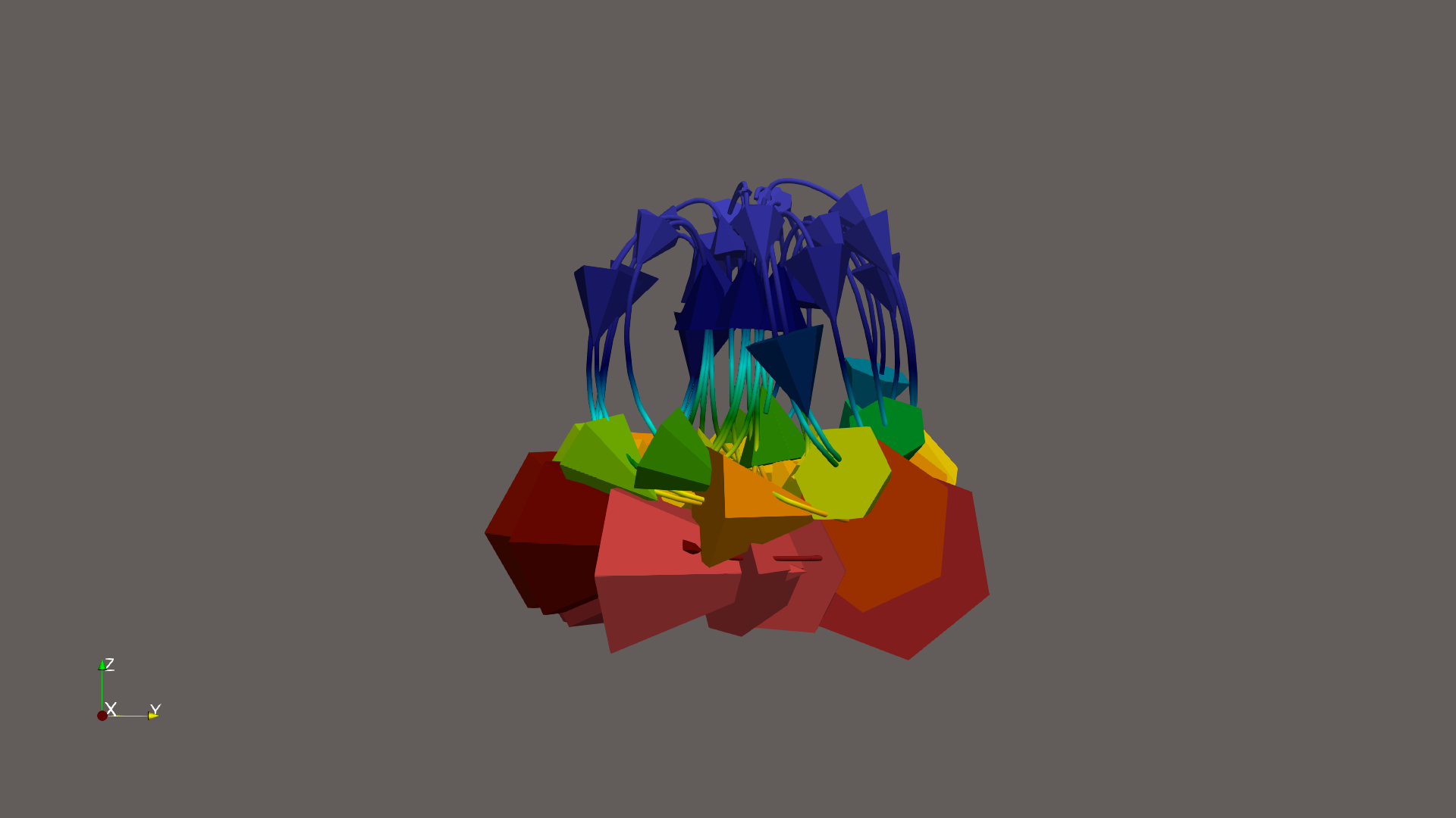
📝 stream-glyph

37/55 (67.3%)

📋 Task Description

I would like to use ParaView to visualize a dataset. Read in the file named "stream-glyph/data/stream-glyph.ex2". Trace streamlines of the V data array seeded from a default point cloud. Render the streamlines with tubes. Add cone glyphs to the streamlines. Color the streamlines and glyphs by the Temp data array. View the result in the +X direction. Save a screenshot of the result in the filename "stream-glyph/results/{agent_mode}/stream-glyph.png". The rendered view and saved screenshot should be 1920 x 1080 pixels. (Optional, but must save if use paraview) Save the paraview state as "stream-glyph/results/{agent_mode}/stream-glyph.pvsm". (Optional, but must save if use python script) Save the python script as "stream-glyph/results/{agent_mode}/stream-glyph.py". Do not save any other files, and always save the visualization image.

🖼️ Visualization Comparison

Ground Truth

Agent Result

📏 Vision Evaluation Rubrics

Score Summary

Total Score

22/40

Goals

4

Points/Goal

10

Goal 1

6/10

Criterion: Streamline Generation: Are streamlines properly traced following the V variable flow field with appropriate seeding from the point cloud?

Judge's Assessment: The ground truth shows a dense bundle of smoothly arcing streamlines seeded from a point cloud, forming a coherent dome-like structure. The result image does show streamlines that arc upward in a similar overall pattern, but there are noticeably fewer lines and the structure is much sparser/less continuous, suggesting different seeding density or integration settings.

Goal 2

4/10

Criterion: Tube and Glyph Rendering: Are streamlines rendered as tubes with cone glyphs properly attached showing flow direction and magnitude?

Judge's Assessment: In the ground truth, streamlines are clearly rendered as tubes and have many small cone glyphs distributed along them. In the result, the streamlines appear as thin lines (not tube-like), and the glyphs are very large, blocky cone-like shapes that dominate the image and do not appear properly attached/distributed along the streamlines in the same way as the reference.

Goal 3

5/10

Criterion: Temperature Color Mapping: Are both streamlines and glyphs correctly colored by the Temp variable with appropriate color scaling?

Judge's Assessment: The ground truth uses a Temp-based diverging scheme (red/orange at the bottom transitioning to white/blue at the top) consistently on both tubes and cones. The result uses a rainbow/jet-like colormap (red-yellow-green-cyan-blue) and the streamlines/glyphs coloring does not match the reference Temp appearance or scaling; additionally the oversized glyphs obscure much of the colored streamlines.

Goal 4

7/10

Criterion: View Configuration: Is the visualization displayed from the correct +x view direction providing clear visibility of the flow patterns and structures?

Judge's Assessment: The +X view in the ground truth presents a symmetric front view of the arcing streamlines. The result view is broadly similar (x-axis indicator suggests a comparable orientation), but the camera appears slightly offset/zoomed and the model is not framed or centered like the ground truth, with a different background color further reducing the match.

Overall Assessment

The result captures the general idea of upward-curving streamlines from a point-cloud seed and roughly the +X viewing orientation, but it significantly diverges from the expected rendering: streamlines are not shown as tubes, cone glyphs are incorrectly scaled/placed, and the temperature colormap/scaling does not match the ground truth.

📊 Detailed Metrics

Visualization Quality

22/40

Output Generation

5/5

Efficiency

10/10

Completed in 41.25 seconds (excellent)

📝 subseries-of-time-series

27/45 (60.0%)

📋 Task Description

Read the file "subseries-of-time-series/data/subseries-of-time-series.ex2". Load two element blocks: the first is called 'Unnamed block ID: 1 Type: HEX', the second is called 'Unnamed block ID: 2 Type: HEX'. Next, slice this object with a plane with origin at [0.21706008911132812, 4.0, -5.110947132110596] and normal direction [1.0, 0.0, 0.0]. The plane should have no offset. Next, save this time series to a collection of .vtm files. The base file name for the time series is "subseries-of-time-series/results/{agent_mode}/canslices.vtm" and the suffix is '_%d'. Only save time steps with index between 10 and 20 inclusive, counting by 3. Next, load the files "subseries-of-time-series/results/{agent_mode}/canslices_10.vtm", "subseries-of-time-series/results/{agent_mode}/canslices_13.vtm", "subseries-of-time-series/results/{agent_mode}/canslices_16.vtm", and "subseries-of-time-series/results/{agent_mode}/canslices_19.vtm" in multi-block format. Finally, show the multi-block data set you just loaded. Save a screenshot to the file "subseries-of-time-series/results/{agent_mode}/subseries-of-time-series.png". (Optional, but must save if use paraview) Save the paraview state as "subseries-of-time-series/results/{agent_mode}/subseries-of-time-series.pvsm". (Optional, but must save if use python script) Save the python script as "subseries-of-time-series/results/{agent_mode}/subseries-of-time-series.py". Do not save any other files, and always save the visualization image.

🖼️ Visualization Comparison

Ground Truth

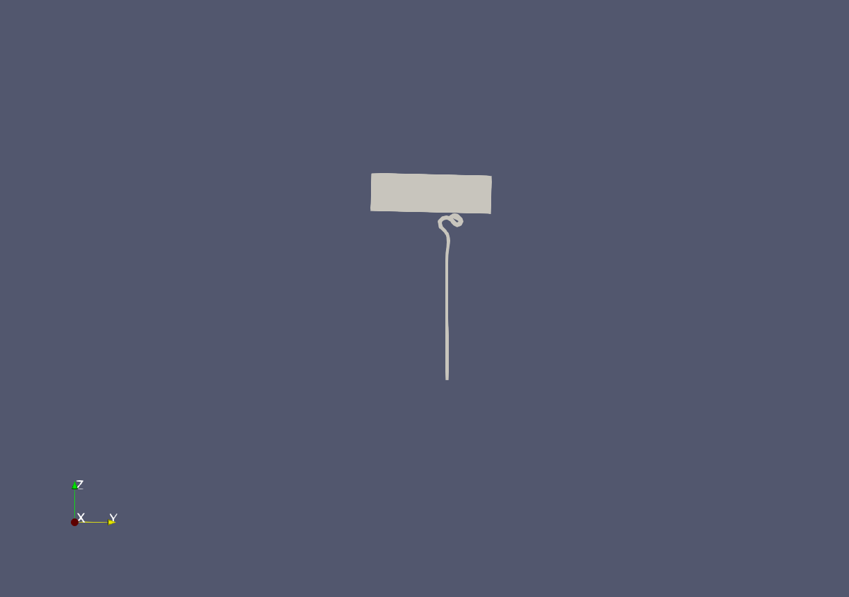
Agent Result

📏 Vision Evaluation Rubrics

Score Summary

Total Score

14/30

Goals

3

Points/Goal

10

Goal 1

4/10

Criterion: Data Loading and Block Selection: Are the specified element blocks properly loaded and the slice plane correctly applied?

Judge's Assessment: Ground truth shows a thin, light-colored sliced cross-section with a small curled feature and a long thin vertical segment beneath a short horizontal bar. The result instead shows a large opaque blue rectangular slice plane with additional geometry extruding to the right. This indicates the slice operation is not matching the expected plane placement/orientation and/or the displayed representation is not the sliced intersection as in the ground truth (it looks more like showing a full plane/large polygonal patch rather than the intended cut geometry).

Goal 2

6/10

Criterion: Multi-block Loading: Are the exported VTM files successfully loaded back as a multi-block dataset?

Judge's Assessment: The result appears to come from loading some VTM output (a multiblock-like combined object is visible), but there is no visual evidence of multiple time-step slices being combined/overlaid as a subseries (10, 13, 16, 19). It looks like a single dominant slice surface rather than a multi-file multiblock set of several similar slices. So multiblock loading is plausible but not clearly correct.

Goal 3

4/10

Criterion: Final Visualization: Is the multi-block dataset properly displayed showing the sliced geometry from the time series?

Judge's Assessment: Final visualization does not resemble the ground truth: the ground truth has small, thin slice geometry with a specific silhouette; the result shows a large solid blue slab and different apparent geometry/scale and camera framing. Even if the data is present, the display is not showing the expected sliced geometry from the time subseries in the same way.

Overall Assessment

The agent result diverges strongly from the expected sliced-cross-section appearance: it displays a large blue planar surface and different geometry orientation/scale compared to the ground truth. Multiblock/time-subseries loading is not clearly demonstrated visually. Overall, the core requirements (correct slice and correct displayed subseries) appear only partially met.

📊 Detailed Metrics

Visualization Quality

14/30

Output Generation

5/5

Efficiency

8/10

Completed in 170.01 seconds (good)

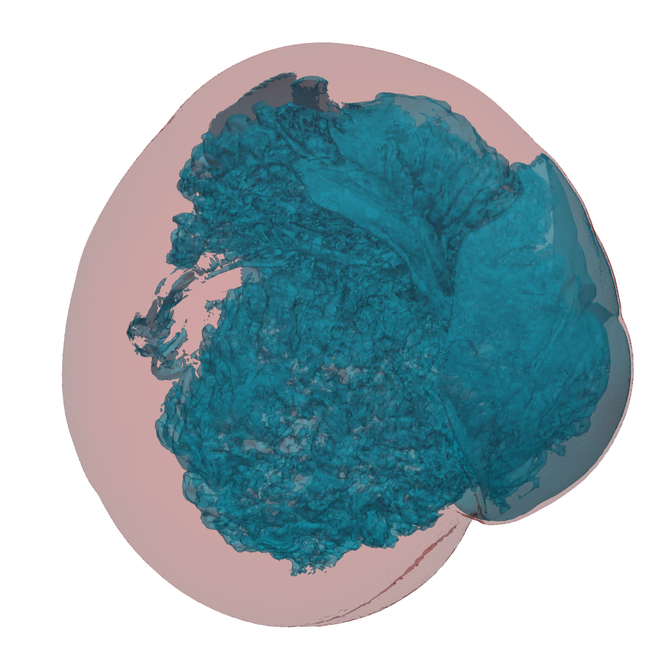
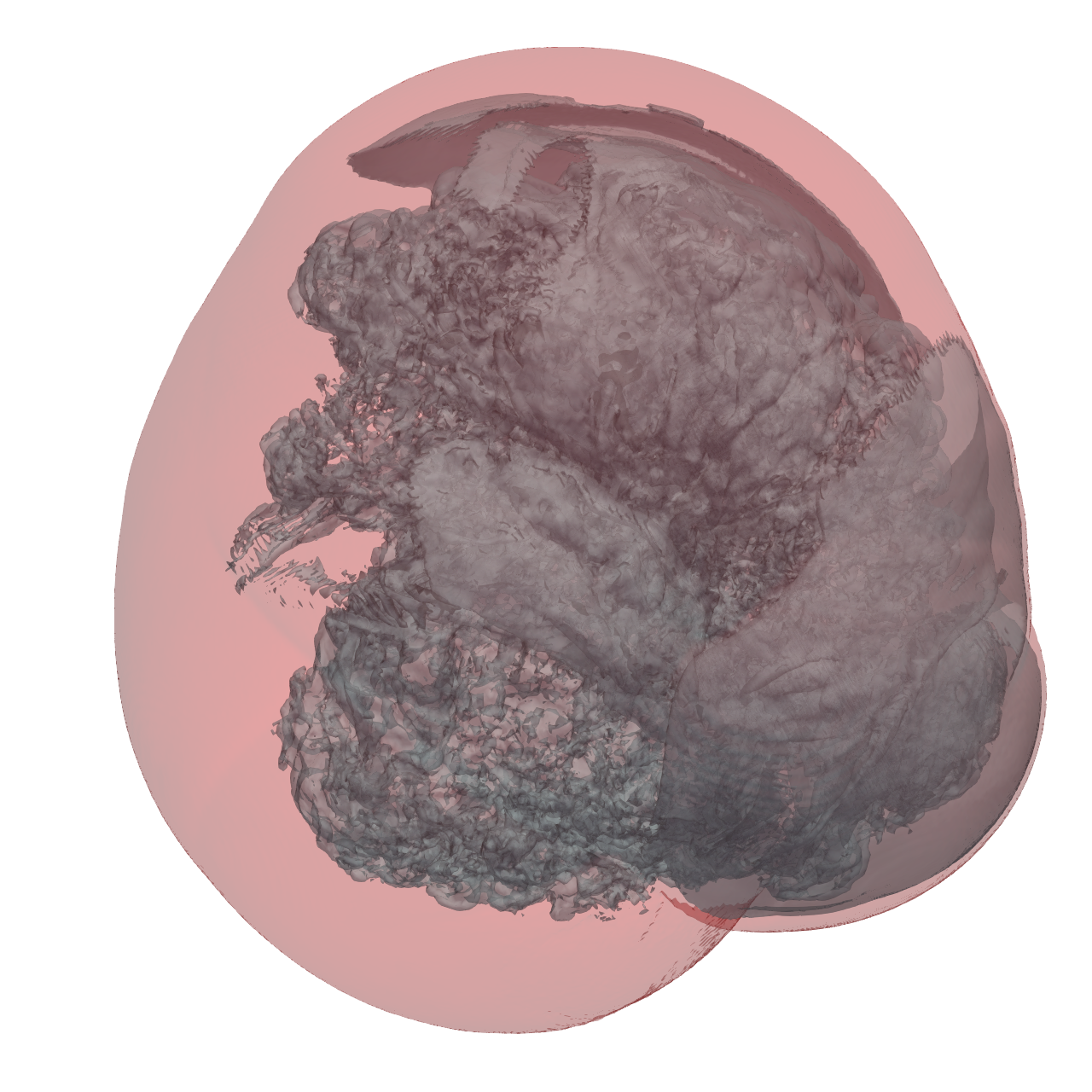
📝 supernova_isosurface

32/45 (71.1%)

📋 Task Description

Task: Load the supernova dataset from "supernova_isosurface/data/supernova_isosurface_256x256x256_float32.raw", the information about this dataset: supernova (Scalar) Data Scalar Type: float Data Byte Order: little Endian Data Spacing: 1x1x1 Data Extent: 256x256x256 Data loading is very important, make sure you correctly load the dataset according to their features. Then visualize it and extract two isosurfaces. One of them use color red, showing areas with low density (isovalue 40 and opacity 0.2), while the other use color light blue, showing areas with high density (isovalue 150 and opacity 0.4). Please think step by step and make sure to fulfill all the visualization goals mentioned above. Only make the two isosurfaces visible. Use a white background. Find an optimal view. Render at 1280x1280. Do not show a color bar or coordinate axes. Set the viewpoint parameters as: [567.97, 80.17, 167.28] to position; [125.09, 108.83, 121.01] to focal point; [-0.11, -0.86, 0.50] to camera up direction. Save the visualization image as "supernova_isosurface/results/{agent_mode}/supernova_isosurface.png". (Optional, but must save if use paraview) Save the paraview state as "supernova_isosurface/results/{agent_mode}/supernova_isosurface.pvsm". (Optional, but must save if use pvpython script) Save the python script as "supernova_isosurface/results/{agent_mode}/supernova_isosurface.py". (Optional, but must save if use VTK) Save the cxx code script as "supernova_isosurface/results/{agent_mode}/supernova_isosurface.cxx" Do not save any other files, and always save the visualization image.

🖼️ Visualization Comparison

Ground Truth

Agent Result

📏 Vision Evaluation Rubrics

Score Summary

Total Score

18/30

Goals

3

Points/Goal

10

Goal 1

6/10

Criterion: Overall Visualization Goal: How well does the result achieve the overall goal of showing the supernova structure with two distinct isosurfaces representing different density regions?

Judge's Assessment: The ground truth shows two clearly distinguishable nested isosurfaces: a translucent red outer low-density shell and a more opaque light-blue inner high-density structure with strong contrast against the white background. In the result, the overall supernova shape and layering are present, but the inner surface appears grayish and low-contrast rather than clearly light blue, making the two-surface separation less visually distinct than in the ground truth.

Goal 2

8/10

Criterion: Does the red isosurface show low density areas (outside regions) with lower opacity?

Judge's Assessment: The low-density isosurface in the result appears as a large, translucent reddish/pink outer shell similar to the ground truth, consistent with a low-opacity red surface. Opacity and extent look broadly correct, though the red reads slightly more pink and the blending with the inner surface reduces clarity compared to the ground truth.

Goal 3

4/10

Criterion: Does the blue isosurface show high density areas (inside regions) with higher opacity?

Judge's Assessment: In the ground truth, the high-density isosurface is distinctly light blue/cyan and noticeably more opaque than the red shell. In the result, the corresponding inner structure is rendered mostly gray/dark and does not read as light blue; its opacity also appears closer to the red shell due to the muted color/contrast. The high-density isosurface is present geometrically but fails the intended color/visibility match.

Overall Assessment

The result captures the general two-ագույն supernova isosurface structure with an outer translucent red shell, but the high-density isosurface does not match the required light-blue appearance and stands out much less than in the ground truth, reducing the effectiveness of the intended two-surface visualization.

📊 Detailed Metrics

Visualization Quality

18/30

Output Generation

5/5

Efficiency

9/10

Completed in 71.99 seconds (very good)

PSNR

22.84 dB

SSIM

0.9762

LPIPS

0.0605

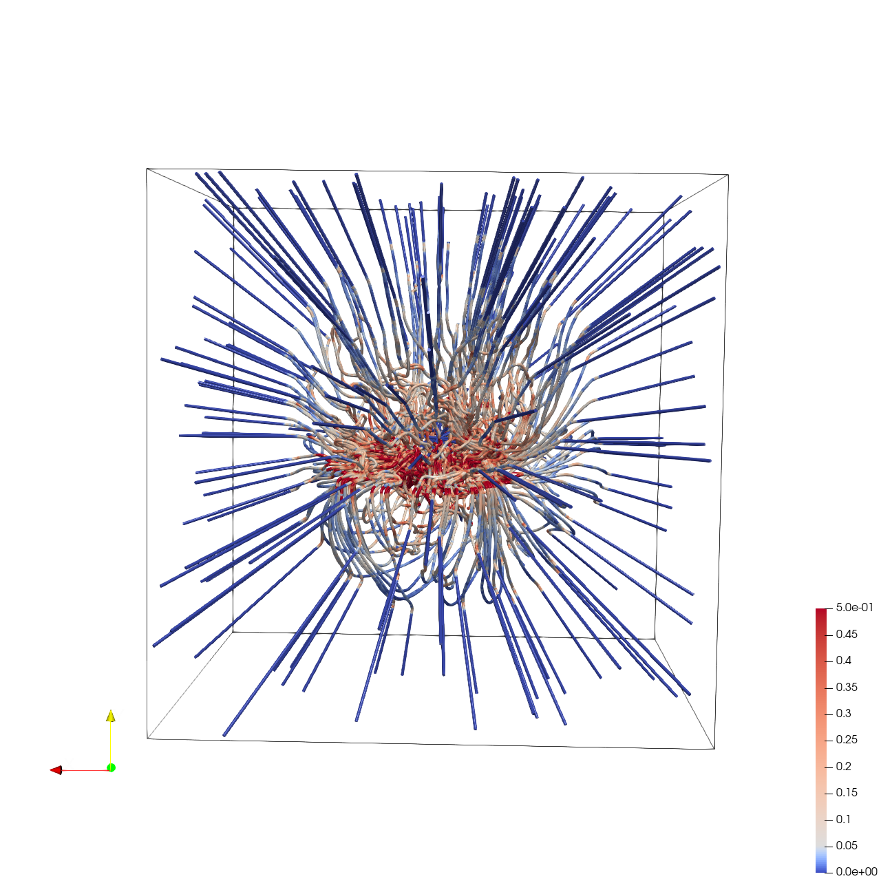
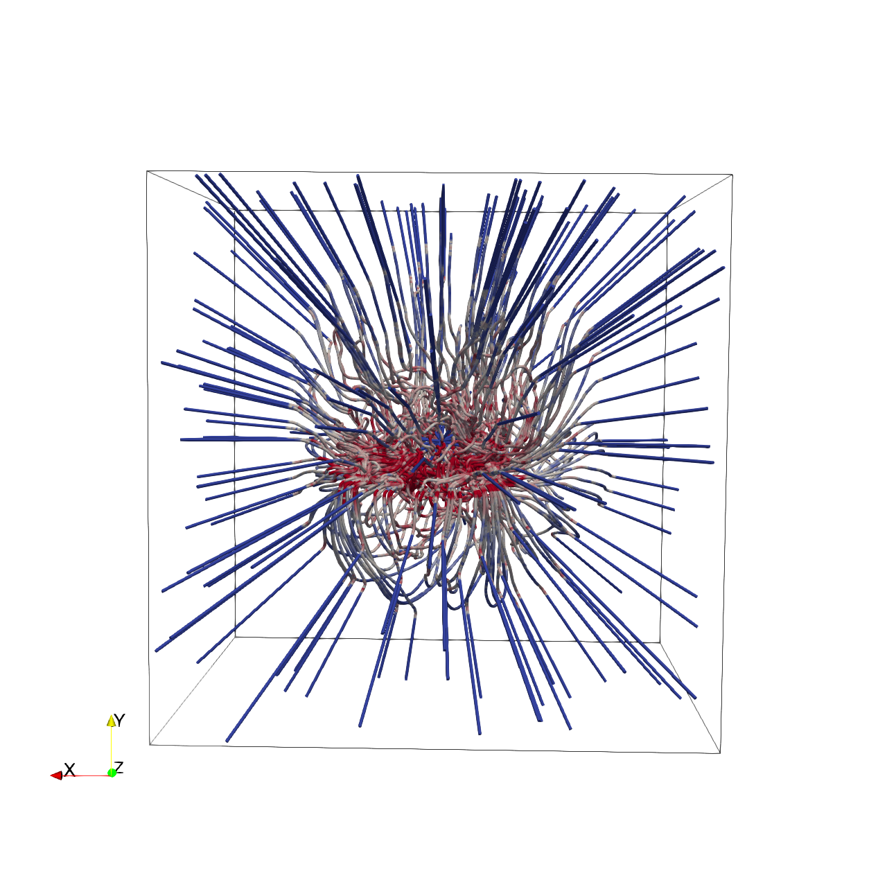
📝 supernova_streamline

42/45 (93.3%)

📋 Task Description

Load the Supernova velocity vector field from "supernova_streamline/data/supernova_streamline_100x100x100_float32_scalar3.raw", the information about this dataset: Supernova Velocity (Vector) Data Scalar Type: float Data Byte Order: Little Endian Data Extent: 100x100x100 Number of Scalar Components: 3 Data loading is very important, make sure you correctly load the dataset according to their features. Create streamlines using a "Stream Tracer" filter with "Point Cloud" seed type. Set the seed center to [50, 50, 50], with 200 seed points and a radius of 45.0. Set maximum streamline length to 100.0. Add a "Tube" filter on the stream tracer. Set tube radius to 0.3 with 12 sides. Color the tubes by Vorticity magnitude using a diverging colormap with the following RGB control points: - Value 0.0 -> RGB(0.231, 0.298, 0.753) (blue) - Value 0.05 -> RGB(0.865, 0.865, 0.865) (white) - Value 0.5 -> RGB(0.706, 0.016, 0.149) (red) Show the dataset bounding box as an outline (black). In the pipeline browser panel, hide the stream tracer and only show the tube filter and the outline. Use a white background. Render at 1280x1280. Set the viewpoint parameters as: [41.38, 73.91, -282.0] to position; [49.45, 49.50, 49.49] to focal point; [0.01, 1.0, 0.07] to camera up direction. Save the visualization image as "supernova_streamline/results/{agent_mode}/supernova_streamline.png". (Optional, but must save if use paraview) Save the paraview state as "supernova_streamline/results/{agent_mode}/supernova_streamline.pvsm". (Optional, but must save if use pvpython script) Save the python script as "supernova_streamline/results/{agent_mode}/supernova_streamline.py". (Optional, but must save if use VTK) Save the cxx code script as "supernova_streamline/results/{agent_mode}/supernova_streamline.cxx" Do not save any other files, and always save the visualization image.

🖼️ Visualization Comparison

Ground Truth

Agent Result

📏 Vision Evaluation Rubrics

Score Summary

Total Score

29/30

Goals

3

Points/Goal

10

Goal 1

10/10

Criterion: Central Structure: Is there a dense, chaotic cluster of streamlines near the center of the volume, matching the ground truth?

Judge's Assessment: The result shows a dense, chaotic bundle of streamline tubes concentrated around the volume center, with strong visual similarity to the ground truth’s central tangled structure (same overall density and spatial placement).

Goal 2

10/10

Criterion: Radial Extensions: Are there long, straight streamline tubes extending radially outward from the central region, similar to the ground truth?

Judge's Assessment: Long, mostly straight tubes extend radially outward from the central region in many directions, matching the ground truth pattern in both extent and distribution (including prominent outward spokes reaching near the bounding box).

Goal 3

9/10

Criterion: Color Mapping: Are the tubes colored by vorticity magnitude using a blue-white-red diverging colormap, with warm colors concentrated near the center and cool colors on the extended lines?

Judge's Assessment: Coloring matches the intended diverging blue–white–red mapping: cooler blues dominate the long outer radial lines while warmer reds concentrate in the central high-vorticity region, with light/neutral tones in between. Minor differences in exact saturation/contrast relative to the ground truth are visible but do not change the qualitative mapping.

Overall Assessment

Overall, the result closely matches the ground truth: correct central turbulent cluster, correct radial spoke-like extensions, and appropriate vorticity-based blue–white–red diverging coloration with warm center and cool periphery. Only slight color/contrast differences are apparent.

📊 Detailed Metrics

Visualization Quality

29/30

Output Generation

5/5

Efficiency

8/10

Completed in 174.74 seconds (good)

PSNR

15.91 dB

SSIM

0.8532

LPIPS

0.2938

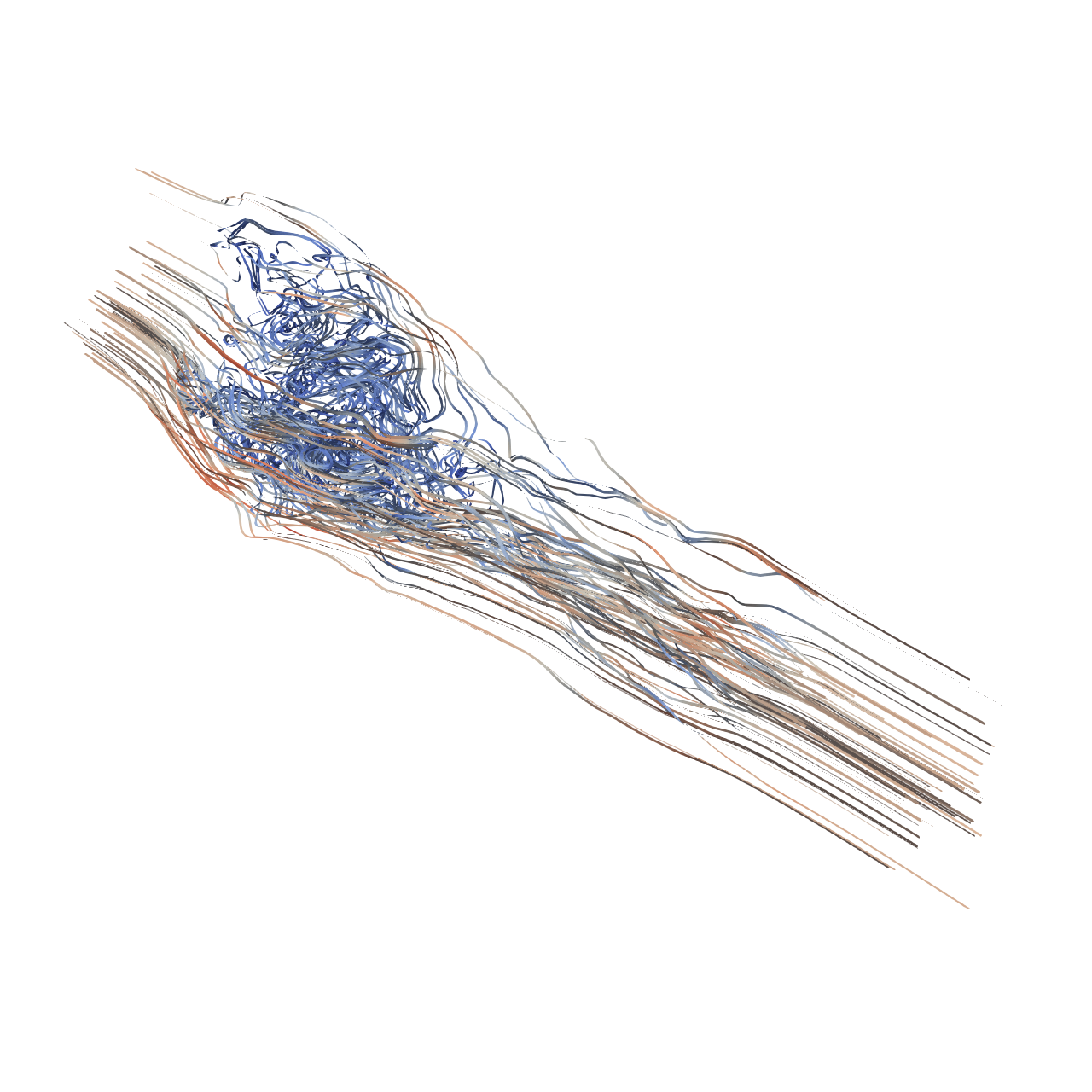
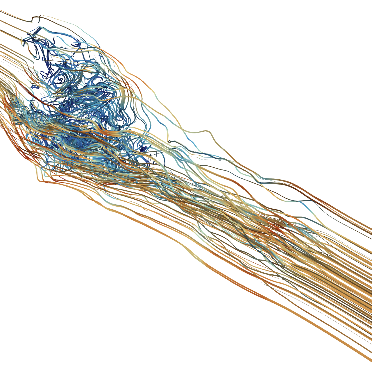
📝 tangaroa_streamribbon

45/55 (81.8%)

📋 Task Description

Task: Load the tangaroa dataset from "tangaroa_streamribbon_300x180x120_float32_scalar3.raw", the information about this dataset: tangaroa (Vector) Data Scalar Type: float Data Byte Order: little Endian Data Extent: 300x180x120 Number of Scalar Components: 3 Data loading is very important, make sure you correctly load the dataset according to their features. Apply "streamline tracer" filter, set the "Seed Type" to point cloud, turn off the "show sphere", set the center to [81.6814, 80.708, 23.5093], and radius to 29.9 Add "Ribbon" filter to the streamline tracer results and set width to 0.3, set the Display representation to Surface. In pipeline browser panel, hide everything except the ribbon filter results. Please think step by step and make sure to fulfill all the visualization goals mentioned above. Use a white background. Find an optimal view. Render at 1280x1280. Do not show a color bar or coordinate axes. Set the viewpoint parameters as: [372.27, 278.87, 214.44] to position; [169.85, 76.46, 12.02] to focal point; [-0.41, 0.82, -0.41] to camera up direction. Save the visualization image as "tangaroa_streamribbon/results/{agent_mode}/tangaroa_streamribbon.png". (Optional, but must save if use paraview) Save the paraview state as "tangaroa_streamribbon/results/{agent_mode}/tangaroa_streamribbon.pvsm". (Optional, but must save if use pvpython script) Save the python script as "tangaroa_streamribbon/results/{agent_mode}/tangaroa_streamribbon.py". (Optional, but must save if use VTK) Save the cxx code script as "tangaroa_streamribbon/results/{agent_mode}/tangaroa_streamribbon.cxx" Do not save any other files, and always save the visualization image.

🖼️ Visualization Comparison

Ground Truth

Agent Result

📏 Vision Evaluation Rubrics

Score Summary

Total Score

34/40

Goals

4

Points/Goal

10

Goal 1

9/10

Criterion: Overall Visualization Goal: Does the result match the ground truth visualization of tangaroa flow structures using ribbon surfaces?

Judge's Assessment: The result shows ribbon-like streamline surfaces on a white background with no visible axes or color bar, matching the intended streamribbon visualization goal. The overall structure (a dense swirling region on the left feeding into long downstream ribbons to the right) matches the ground truth very closely. Minor differences in thickness/opacity and color mapping keep it from being a perfect match.

Goal 2

9/10

Criterion: Flow Surface Patterns: Do the ribbon surfaces show similar flow patterns and structures as the ground truth?

Judge's Assessment: Flow patterns are highly consistent with the ground truth: a compact recirculating/tangled cluster in the upper-left region and multiple coherent ribbon trajectories stretching diagonally down-right. The main vortical shapes and overall curvature/trajectory families are very similar, with only small deviations in the density/visibility of some strands.

Goal 3

8/10

Criterion: Surface Coverage: Is the spatial distribution and coverage of the flow surfaces similar to the ground truth?

Judge's Assessment: Spatial coverage largely matches: similar concentration near the left swirling core and comparable downstream extent. The result image appears slightly more filled/dense in the midstream region (more visible ribbons and thicker-looking bands), which changes the perceived coverage compared to the somewhat sparser ground truth depiction.

Goal 4

8/10

Criterion: Visual Appearance: Do the ribbon surfaces appear similar in width and structure to the ground truth?

Judge's Assessment: Ribbons appear as surface bands with a generally consistent width, resembling the ground truth. However, the result looks a bit thicker/more opaque overall, and the color palette differs (more green/teal tones and stronger saturation) versus the ground truth’s more muted gray/brown with blue/orange accents, affecting perceived ribbon structure and separation.

Overall Assessment

The result is an excellent match to the ground truth: same camera framing and the characteristic tangaroa streamribbon morphology (left-side turbulent swirl feeding long downstream ribbons). Differences are limited to styling—slightly higher ribbon density/thickness/opacity and a different color mapping—so the core visualization requirements are met very well.

📊 Detailed Metrics

Visualization Quality

34/40

Output Generation

5/5

Efficiency

6/10

Completed in 254.40 seconds (slow)

PSNR

25.64 dB

SSIM

0.9576

LPIPS

0.0248

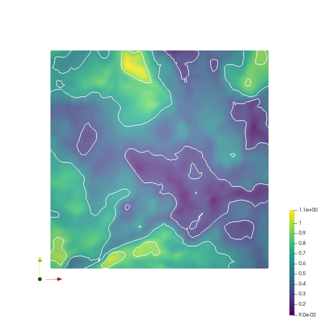
📝 tgc-velocity_contour

45/55 (81.8%)

📋 Task Description

Load the turbulence-gravity-cooling velocity field dataset from "tgc-velocity_contour/data/tgc-velocity_contour.vti" (VTI format, 64x64x64). Extract a slice at z=32 and color it by velocity magnitude using 'Viridis (matplotlib)' colormap. Also add contour lines of velocity magnitude on the same slice at values [0.3, 0.6, 0.9, 1.2] using the Contour filter on the slice output. Display contour lines in white. Add a color bar labeled 'Velocity Magnitude'. Light gray background (RGB: 0.9, 0.9, 0.9). Top-down camera. Render at 1024x1024. Set the viewpoint parameters as: [31.5, 31.5, 100.0] to position; [31.5, 31.5, 32.0] to focal point; [0.0, 1.0, 0.0] to camera up direction. Save the visualization image as "tgc-velocity_contour/results/{agent_mode}/tgc-velocity_contour.png". (Optional, but must save if use paraview) Save the paraview state as "tgc-velocity_contour/results/{agent_mode}/tgc-velocity_contour.pvsm". (Optional, but must save if use pvpython script) Save the python script as "tgc-velocity_contour/results/{agent_mode}/tgc-velocity_contour.py". (Optional, but must save if use VTK) Save the cxx code script as "tgc-velocity_contour/results/{agent_mode}/tgc-velocity_contour.cxx" Do not save any other files, and always save the visualization image.

🖼️ Visualization Comparison

Ground Truth

Agent Result

📏 Vision Evaluation Rubrics

Score Summary

Total Score

30/40

Goals

4

Points/Goal

10

Goal 1

8/10

Criterion: Overall Visualization Goal: Does the result match the ground truth slice and contour visualization of the TGC velocity field?

Judge's Assessment: Result shows a z-slice colored with a Viridis-like colormap, overlaid with white contour lines and a vertical colorbar labeled “Velocity Magnitude”, matching the intended visualization type. However, the framing/camera differs: the result is zoomed in/cropped to a subregion compared to the ground truth’s more complete slice view, and the background appears darker (not the light gray 0.9,0.9,0.9 seen in the ground truth).

Goal 2

7/10

Criterion: Slice Pattern: Does the colored slice show similar patterns and structures as the ground truth?

Judge's Assessment: The slice pattern broadly resembles the ground truth (large purple low-velocity region with surrounding teal/green and some yellow areas), but because the result is significantly zoomed/cropped, the global spatial arrangement and full-extent structures visible in the ground truth are not reproduced.

Goal 3

7/10

Criterion: Contour Lines: Are the contour lines positioned and shaped similarly to the ground truth?

Judge's Assessment: Contour lines are present and white, and their shapes in the visible central region are consistent with the ground truth’s major contours (e.g., the large enclosing contour around the central low-velocity region and a nested loop). But due to zoom/cropping, many contours present in the full slice are missing from view, making the overall contour placement less comparable.

Goal 4

8/10

Criterion: Color Mapping: Is the color distribution on the slice visually similar to the ground truth?

Judge's Assessment: Color mapping looks consistent with Viridis and the value range on the colorbar appears similar to the ground truth. The distribution of colors within the shown region matches reasonably well, though the different zoom and slightly different overall brightness/background reduce the perceived similarity.

Overall Assessment

The result largely achieves the correct slice+contour visualization with appropriate colormap, white contours, and labeled colorbar. The main discrepancies versus ground truth are the camera/framing (result is zoomed/cropped rather than showing the full slice) and the background tone, which together reduce overall match quality despite locally similar slice/contour structure.

📊 Detailed Metrics

Visualization Quality

30/40

Output Generation

5/5

Efficiency

10/10

Completed in 56.64 seconds (excellent)

PSNR

21.13 dB

SSIM

0.9676

LPIPS

0.0470

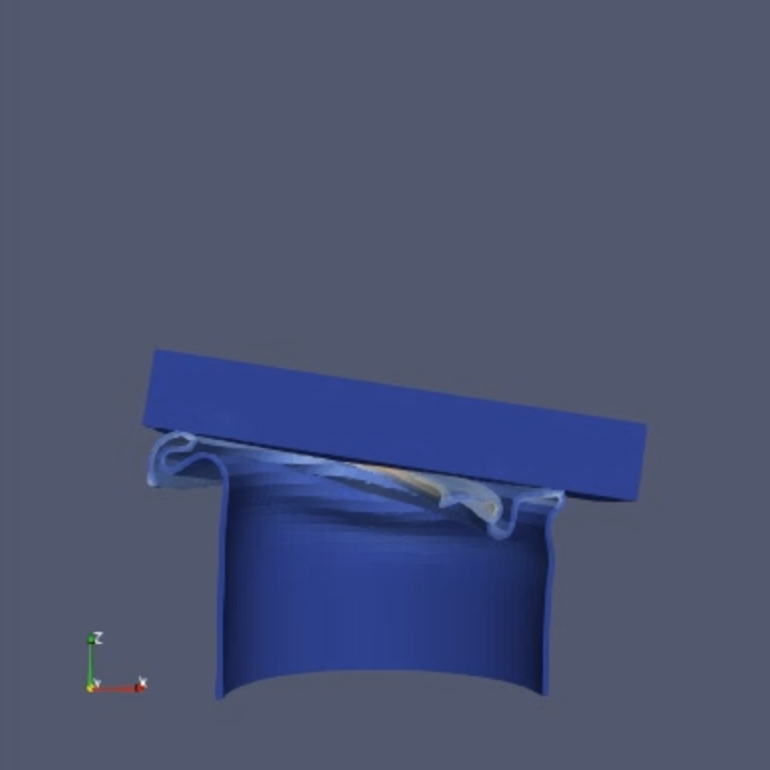
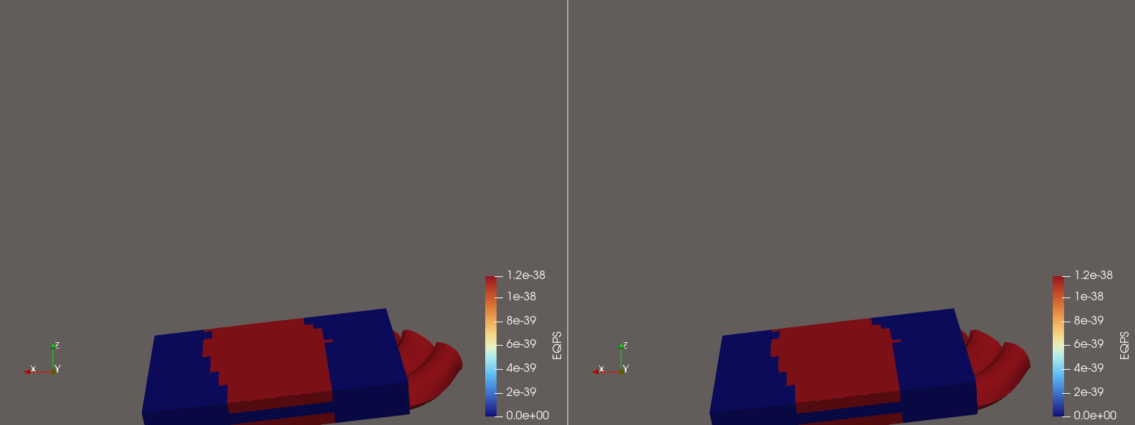
📝 time-varying

34/55 (61.8%)

📋 Task Description

Read the dataset in the file "time-varying/data/time-varying.ex2", and color the data by the EQPS variable. Viewing in the +y direction, play an animation through the time steps, with visible color bar legend. Rescale the data range to last time step, and play the animation again. Create a second linked render view to the right of the first, applying a temporal interpolator to the second view. Play the animation simultaneously in both views, and save the animation of both views in "time-varying/results/{agent_mode}/time-varying.avi". Print the following statistics: average value of EQPS over all locations and all time steps, average value of EQPS over all locations in the first half of the time steps, average value of EQPS over all locations in the even numbered time steps, and variance of EQPS over all locations and all the time steps. Save the last frame of the visualization image as "time-varying/results/{agent_mode}/time-varying.png". (Optional, but must save if use paraview) Save the paraview state as "time-varying/results/{agent_mode}/time-varying.pvsm". (Optional, but must save if use python script) Save the python script as "time-varying/results/{agent_mode}/time-varying.py". Do not save any other files, and always save the visualization image.

🖼️ Visualization Comparison

Ground Truth

Agent Result

📏 Vision Evaluation Rubrics

Score Summary

Total Score

21/40

Goals

4

Points/Goal

10

Goal 1

2/10

Criterion: Temporal Animation Quality: Does the animation smoothly progress through all time steps showing the evolution of the EQPS variable over time?

Judge's Assessment: Only a single static frame is provided for the result, so smooth progression through time steps and the required second playback (after rescaling range to last time step) cannot be verified. The ground truth indicates a time-varying field with visible internal structure, which is not demonstrably reproduced via animation here.

Goal 2

6/10

Criterion: Dual View Configuration: Are both render views properly configured with the second view showing temporal interpolation effects compared to the first?

Judge's Assessment: The result shows two side-by-side render views with the same dataset and separate color bars, matching the requested dual-view layout. However, there is no visible difference between left and right views that would indicate temporal interpolation being applied in the second view (they look identical in color pattern and geometry), whereas the task expects the second view to show interpolated temporal behavior relative to the first.

Goal 3

7/10

Criterion: Color Mapping and Legend: Is the EQPS variable properly color-mapped with an appropriate color bar legend visible throughout the animation?

Judge's Assessment: A color bar legend labeled "EQPS" is visible in both result views, satisfying the legend requirement. However, the color mapping/appearance differs notably from the ground truth: the ground truth shows a largely blue surface with lighter internal/edge features, while the result shows large saturated red regions and a very different overall distribution. This suggests a mismatch in colormap range/rescaling behavior and/or lighting/representation compared to the reference.

Goal 4

6/10

Criterion: View Direction and Layout: Is the +y direction view properly set and are both views arranged side-by-side in the correct layout configuration?

Judge's Assessment: The two views are arranged side-by-side as required. The orientation appears roughly consistent between both result views, but it does not match the ground truth camera/view direction (+y) well: the ground truth shows a more top/side look with different visible surfaces and internal features, while the result shows a different tilt and overall geometry presentation. So layout is correct, but view direction/pose is not a close match.

Overall Assessment

The result succeeds in creating a two-panel layout with EQPS color bars, but it does not match the ground-truth visual appearance of the field, does not demonstrate temporal interpolation differences between the two views, and provides no evidence of the required animation behavior (including rescaled replay). Camera/view direction also deviates from the reference.

📊 Detailed Metrics

Visualization Quality

21/40

Output Generation

5/5

Efficiency

8/10

Completed in 161.87 seconds (good)

📝 tornado

24/45 (53.3%)

📋 Task Description

Load the Tornado vector field from "tornado/data/tornado_64x64x64_float32_scalar3.raw", the information about this dataset: Tornado (Vector) Data Scalar Type: float Data Byte Order: Little Endian Data Extent: 64x64x64 Number of Scalar Components: 3 Data loading is very important, make sure you correctly load the dataset according to their features. Create a streamline visualization using a "Stream Tracer" filter with "Point Cloud" seed type. Set the seed center to [31.5, 31.5, 47.25], radius 12.6, and maximum streamline length to 512.0. Add a "Tube" filter (radius 0.25) on the stream tracer. Color the tubes by Velocity magnitude using the 'Cool to Warm (Diverging)' colormap. Also display the stream tracer directly with line width 5.0 and "Render Lines As Tubes" enabled. Add a "Glyph" filter on the original data using Arrow glyph type. Orient arrows by the Velocity vector and scale by Velocity magnitude with a scale factor of 25.0. Set maximum number of sample points to 2500. Color glyphs by Velocity magnitude using the same colormap. Add an "Outline" filter to display the dataset bounding box (black). Use a white background (RGB: 1.0, 1.0, 1.0). Find an optimal view. Render at 1280x1280. Show both color bar and coordinate axes. Set the viewpoint parameters as: [142.01, -36.46, 93.96] to position; [31.5, 31.5, 31.5] to focal point; [-0.35, 0.25, 0.90] to camera up direction. Save the visualization image as "tornado/results/{agent_mode}/tornado.png". (Optional, but must save if use paraview) Save the paraview state as "tornado/results/{agent_mode}/tornado.pvsm". (Optional, but must save if use pvpython script) Save the python script as "tornado/results/{agent_mode}/tornado.py". (Optional, but must save if use VTK) Save the cxx code script as "tornado/results/{agent_mode}/tornado.cxx" Do not save any other files, and always save the visualization image.

🖼️ Visualization Comparison

Ground Truth

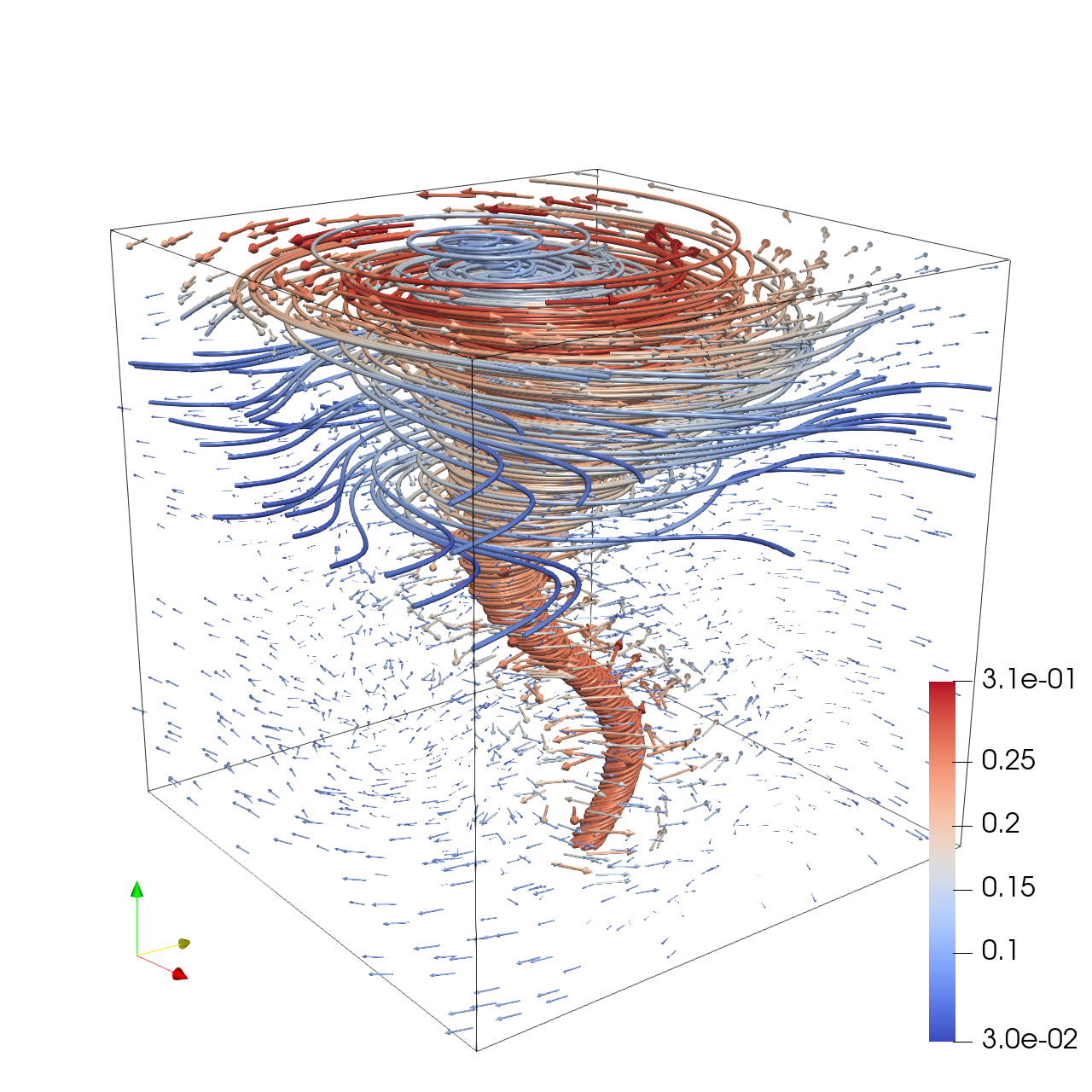
Agent Result

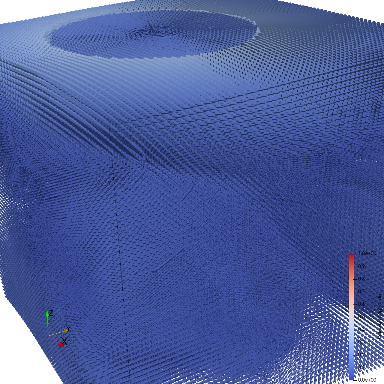
📏 Vision Evaluation Rubrics

Score Summary

Total Score

11/30

Goals

3

Points/Goal

10

Goal 1

2/10

Criterion: Vortex Structure: Is a funnel-shaped vortex core visible with streamlines spiraling around a central vertical axis, matching the ground truth?

Judge's Assessment: Ground truth shows a clear funnel-shaped vortex with streamlines/tubes spiraling around a central vertical core and widening toward the top. The result image does not show a distinct streamline-based funnel; instead it appears dominated by a dense field of small repeated marks (likely glyphs) with no clearly visible spiral streamline structure or central vortex core comparable to the ground truth.

Goal 2

6/10

Criterion: Glyph Presence: Are arrow glyphs distributed throughout the volume showing velocity direction, similar to the ground truth?

Judge's Assessment: Ground truth has arrow glyphs scattered throughout the volume (moderate density, clearly readable arrows). The result contains an extremely dense distribution of arrow-like glyphs covering nearly the entire volume, which indicates glyph presence but at a much higher sampling/density than the reference, reducing similarity and readability.

Goal 3

3/10

Criterion: Color Mapping: Are both the streamline tubes and arrow glyphs colored by velocity magnitude using a blue-to-red diverging colormap, matching the ground truth color distribution?

Judge's Assessment: Ground truth uses a cool-to-warm diverging map with clear variation: blue in lower-speed regions and warm reds/oranges concentrated near the high-speed vortex core/top ring. The result is overwhelmingly blue with little visible warm coloration, suggesting the color mapping/range is not matching the reference (or velocity magnitude not properly used for coloring / range not set appropriately).

Overall Assessment

The submitted visualization does not reproduce the key tornado streamline/tube funnel seen in the ground truth, and the color distribution is largely incorrect (nearly all blue). Glyphs are present but massively over-dense compared to the reference, obscuring structure. Overall it only partially meets the glyph requirement and fails to match the vortex/colormap appearance.

📊 Detailed Metrics

Visualization Quality

11/30

Output Generation

5/5

Efficiency

8/10

Completed in 152.30 seconds (good)

PSNR

12.35 dB

SSIM

0.7591

LPIPS

0.2520

📝 twoswirls_streamribbon

38/45 (84.4%)

📋 Task Description

Load the Two Swirls vector field from "twoswirls_streamribbon/data/twoswirls_streamribbon_64x64x64_float32_scalar3.raw", the information about this dataset: Two Swirls (Vector) Data Scalar Type: float Data Byte Order: Little Endian Data Extent: 64x64x64 Number of Scalar Components: 3 Data loading is very important, make sure you correctly load the dataset according to their features. Create two stream ribbons using "Stream Tracer" filters with "Line" seed type (resolution 25 points each), and apply a "Ribbon" filter (width 2.5) to each: - Stream Ribbon 1: Line seed from [16, 10, 32] to [16, 54, 32]. Ribbon colored solid green (RGB: 0.2, 0.7, 0.3) with opacity 0.35. - Stream Ribbon 2: Line seed from [48, 10, 32] to [48, 54, 32]. Ribbon colored solid blue (RGB: 0.2, 0.4, 0.85) with opacity 0.35. Show the dataset bounding box as an outline (black, opacity 0.3). In the pipeline browser panel, hide all stream tracers and only show the ribbon filters and the outline. Use a white background (RGB: 1.0, 1.0, 1.0). Find an optimal view. Render at 1280x1280. Do not show a color bar or coordinate axes. Set the viewpoint parameters as: [30.51, -154.18, 144.99] to position; [30.51, 31.5, 30.91] to focal point; [0.0, 0.53, 0.85] to camera up direction. Save the visualization image as "twoswirls_streamribbon/results/{agent_mode}/twoswirls_streamribbon.png". (Optional, but must save if use paraview) Save the paraview state as "twoswirls_streamribbon/results/{agent_mode}/twoswirls_streamribbon.pvsm". (Optional, but must save if use pvpython script) Save the python script as "twoswirls_streamribbon/results/{agent_mode}/twoswirls_streamribbon.py". (Optional, but must save if use VTK) Save the cxx code script as "twoswirls_streamribbon/results/{agent_mode}/twoswirls_streamribbon.cxx" Do not save any other files, and always save the visualization image.

🖼️ Visualization Comparison

Ground Truth

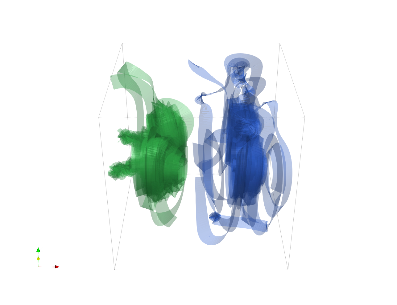
Agent Result

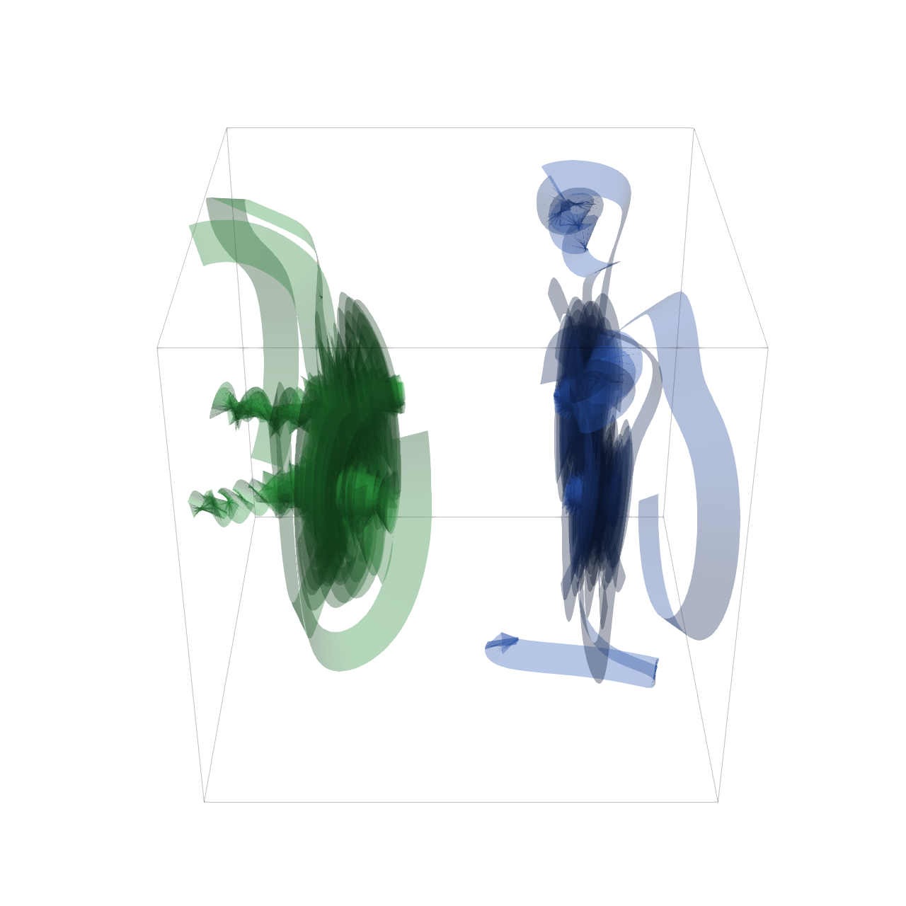
📏 Vision Evaluation Rubrics

Score Summary

Total Score

24/30

Goals

3

Points/Goal

10

Goal 1

9/10

Criterion: Swirl Separation: Are there two visually distinct swirl structures (one on the left and one on the right), matching the spatial arrangement in the ground truth?

Judge's Assessment: Ground truth shows two clearly separated swirl/ribbon structures: a green swirl mass on the left and a blue swirl mass on the right within the bounding box. The result image also shows two distinct structures in the same left/right arrangement with similar spacing. Minor difference: the right (blue) structure in the result is thinner/less filled and appears slightly shifted/compressed compared to the ground truth, but separation and placement are still correct.

Goal 2

7/10

Criterion: Stream Ribbon Shape: Do the ribbon surfaces show wrapped, swirling sheet-like structures similar to the ground truth?

Judge's Assessment: In the ground truth, both ribbons form dense, wrapped, sheet-like swirling surfaces with multiple loops and a substantial core volume (especially the blue on the right). In the result, the left green ribbon still shows a strong swirling sheet with comparable looping, but the right blue ribbon looks less developed: fewer visible wraps, more sparse segments, and a narrower central bundle, so the overall ribbon surface complexity and fullness do not match the ground truth well.

Goal 3

8/10

Criterion: Color and Transparency: Are the stream ribbons rendered with distinct colors (green and blue) and semi-transparency, similar to the ground truth?

Judge's Assessment: Both images use semi-transparent solid green and blue ribbons against a white background, and the colors are clearly distinct. The result appears slightly darker/more opaque in the central ribbon bundles (especially blue) and slightly less uniformly translucent than the ground truth, but overall color assignment and transparency are close.

Overall Assessment

The result correctly captures the key composition: two separated left/right stream ribbons with appropriate green/blue semi-transparent styling inside an outline box. The main discrepancy is geometric: the right (blue) ribbon is noticeably less dense/less fully wrapped than in the ground truth, reducing the similarity of the ribbon surface shape and overall swirl fullness.

📊 Detailed Metrics

Visualization Quality

24/30

Output Generation

5/5

Efficiency

9/10

Completed in 70.43 seconds (very good)

PSNR

21.87 dB

SSIM

0.9056

LPIPS

0.1002

📝 vortex

46/55 (83.6%)

📋 Task Description

Task: Load the vortex dataset from "vortex/data/vortex_128x128x128_float32.raw", the information about this dataset: vortex (Scalar) Data Scalar Type: float Data Byte Order: little Endian Data Extent: 128x128x128 Number of Scalar Components: 1 Instructions: 1. Load the dataset into ParaView. 2. Leverage "contour" filter to achieve iso-surface rendering. In pipeline browser panel, hide everything except the "contour" fileter. 3. In properties panel of "contour" filter, set isosurface value to -0.2, use Solid Color and set the color as beige. 4. Enable Ambient occlusion by toggle the "Use Ambient Occlusion" button in the Render Passes. 5. Add head light with light inspector, set "Coords" as Camera, "Intentsity" to 0.2, Type to "Directional". 6. Use a white background. Find an optimal view. Render at 1280x1280. Do not show a color bar or coordinate axes. 7. Set the viewpoint parameters as: [308.85, 308.85, 308.85] to position; [63.5, 63.5, 63.5] to focal point; [-0.41, 0.82, -0.41] to camera up direction. 8. Save your work: Save the visualization image as "vortex/results/{agent_mode}/vortex.png". (Optional, but must save if use paraview) Save the paraview state as "vortex/results/{agent_mode}/vortex.pvsm". (Optional, but must save if use pvpython script) Save the python script as "vortex/results/{agent_mode}/vortex.py". (Optional, but must save if use VTK) Save the cxx code script as "vortex/results/{agent_mode}/vortex.cxx" Do not save any other files, and always save the visualization image.

🖼️ Visualization Comparison

Ground Truth

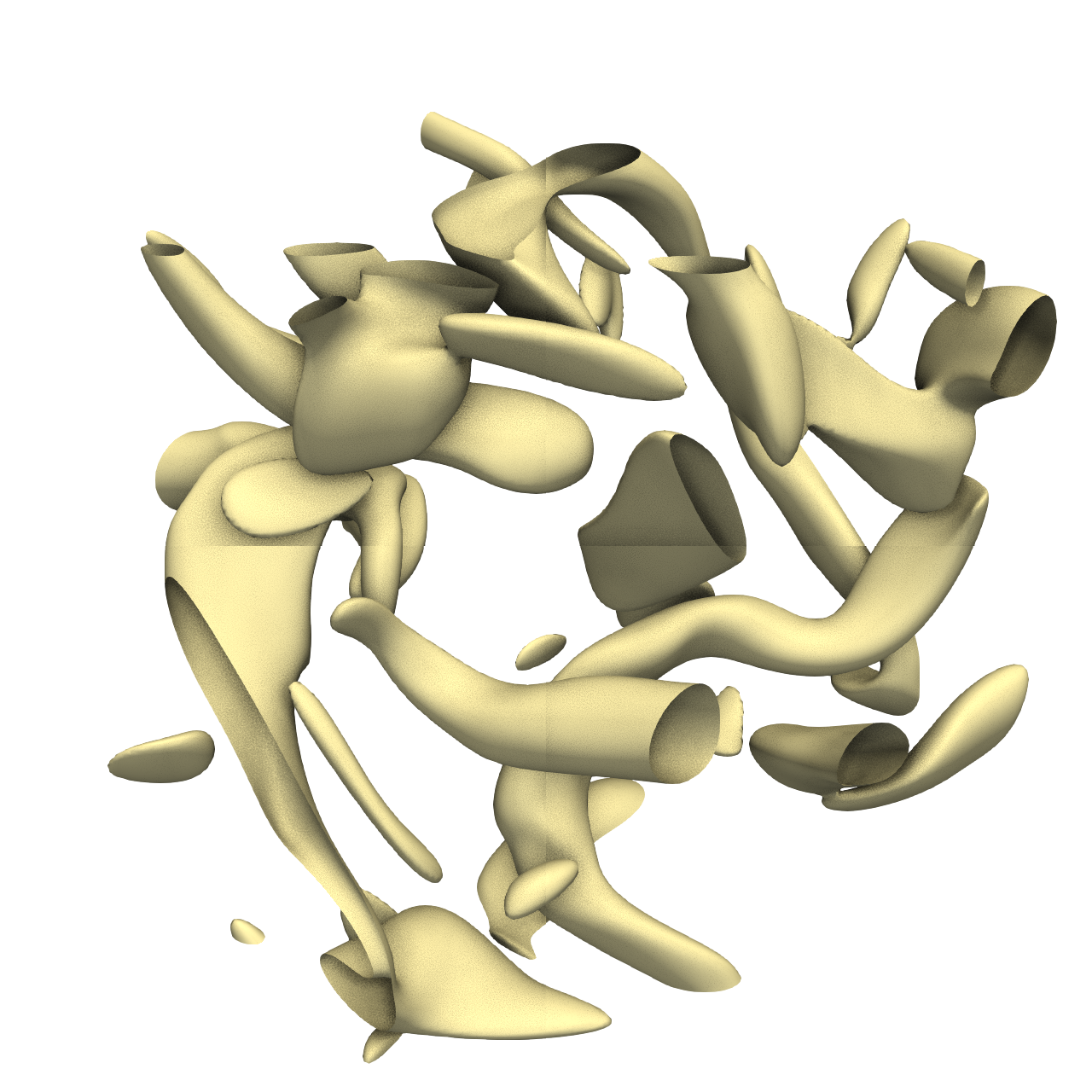
Agent Result

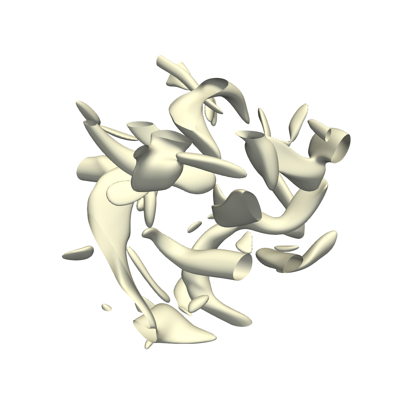
📏 Vision Evaluation Rubrics

Score Summary

Total Score

33/40

Goals

4

Points/Goal

10

Goal 1

9/10

Criterion: Overall Visualization Goal: Does the result match the ground truth isosurface rendering of the vortex scalar field?

Judge's Assessment: The result shows the same overall contour/isosurface rendering of the vortex field as the ground truth: a collection of tubular/sheet-like vortex structures on a white background with no axes or colorbar. The camera framing and general composition are very similar. The main visible difference is surface tone/shading, which makes the result look slightly less like the ground truth’s final render.

Goal 2

9/10

Criterion: Isosurface Structure: Does the isosurface show the same vortex structure and topology as the ground truth?

Judge's Assessment: The isosurface topology and structure closely match the ground truth: same major curled tubes, the large sweeping structure on the right, the thicker cluster on the left, and small detached fragments. No obvious missing or extra large components; minor differences are limited to subtle perceived thickness due to lighting/shading rather than geometry changes.

Goal 3

7/10

Criterion: Surface Appearance: Does the surface color and shading appear similar to the ground truth?

Judge's Assessment: Surface appearance differs noticeably. The ground truth has a warmer beige tone and stronger ambient-occlusion-like shading, giving deeper creases and more contrast. The result appears paler/whiter (less beige) and a bit flatter/less occluded, suggesting differences in solid color choice, lighting intensity, or AO strength.

Goal 4

8/10

Criterion: Visualization Clarity: Are the vortex features clearly visible and comparable to the ground truth?

Judge's Assessment: Vortex features are clear and well-separated, and the white background helps readability. However, compared to the ground truth, the reduced contrast from weaker AO/lighting makes some overlapping surfaces and interior cavities slightly harder to distinguish.

Overall Assessment

Geometrically and compositionally the result is an excellent match to the ground truth isosurface rendering, with the same vortex structures and viewpoint. The main shortcomings are aesthetic/rendering related: the surface color is less beige and the shading/ambient occlusion effect is weaker, reducing depth and contrast compared to the reference.

📊 Detailed Metrics

Visualization Quality

33/40

Output Generation

5/5

Efficiency

8/10

Completed in 159.60 seconds (good)

PSNR

27.43 dB

SSIM

0.9783

LPIPS

0.0410

📝 write-ply

25/45 (55.6%)

📋 Task Description

I would like to use ParaView to visualize a dataset. Create a wavelet object. Change the view size to 400x400. Show the wavelet object and reset the camera to fit the data. Next, create a contour of wavelet object from the dataset "RTData". The contour should have isosurfaces at the following values: 97.222075, 157.09105, 216.96002500000003, and 276.829. Show the contour and color it with the same colormap that is used for coloring "RTData". Finally, save the contour in PLY format to the file "write-ply/results/{agent_mode}/PLYWriterData.ply". Save the visualization image as "write-ply/results/{agent_mode}/write-ply.png". (Optional, but must save if use paraview) Save the paraview state as "write-ply/results/{agent_mode}/write-ply.pvsm". (Optional, but must save if use python script) Save the python script as "write-ply/results/{agent_mode}/write-ply.py". Do not save any other files, and always save the visualization image.

🖼️ Visualization Comparison

Ground Truth

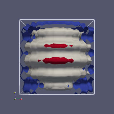
Agent Result

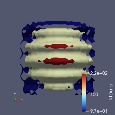
📏 Vision Evaluation Rubrics

Score Summary

Total Score

10/30

Goals

3

Points/Goal

10

Goal 1

2/10

Criterion: Cube Creation: Is the cube object properly created and displayed with correct geometry?

Judge's Assessment: Ground truth shows a multi-layer contour structure (red inner bands, light mid isosurface, dark blue outer fragments) within a box outline—this is consistent with a wavelet contour task, not a cube. The result image also shows the same kind of multi-isosurface contour, but there is no distinct cube geometry created/displayed as a primary object. Thus the cube-creation criterion is largely not addressed (no clear cube surface/edges beyond the dataset bounding box).

Goal 2

1/10

Criterion: PLY Import: Is the exported PLY file correctly loaded back into ParaView maintaining geometric fidelity?

Judge's Assessment: There is no evidence in the result of a PLY being re-imported and displayed as a standalone dataset (e.g., a reloaded mesh with a different source name/appearance). The screenshot only shows the contour rendering with scalar bar; nothing indicates a PLY round-trip import. Compared to ground truth, which also does not depict a cube/PLY import, this criterion is not met.

Goal 3

7/10

Criterion: Visualization Quality: Does the imported cube display properly with correct surface representation and rendering?

Judge's Assessment: Visually, the result matches the ground truth contour rendering fairly well: same overall shape, similar three main isosurface bands and blue outer regions. A noticeable difference is the presence of the RTData scalar bar in the result and slightly different background/lighting, but the surface representation and rendering quality of the shown geometry are still good and consistent with the expected contour appearance.

Overall Assessment

The result closely reproduces the expected contour visualization of the wavelet/RTData (good rendering match), but it does not demonstrate the cube-creation goal nor the PLY export+re-import fidelity checks described in the evaluation criteria. Most credit comes from the visual match of the rendered surface/contour.

📊 Detailed Metrics

Visualization Quality

10/30

Output Generation

5/5

Efficiency

10/10

Completed in 43.26 seconds (excellent)

📊 Overall Performance

Overall Score

Test Cases

Avg Vision Score

PSNR (Scaled)

SSIM (Scaled)

LPIPS (Scaled)

Completion Rate

ℹ️ About Scaled Metrics

🔧 Configuration

📝 ABC

📋 Task Description

🖼️ Visualization Comparison

Ground Truth

Agent Result

📏 Vision Evaluation Rubrics

Score Summary

Overall Assessment

📊 Detailed Metrics

📝 Bernard

📋 Task Description

🖼️ Visualization Comparison

Ground Truth

Agent Result

📏 Vision Evaluation Rubrics

Score Summary

Overall Assessment

📊 Detailed Metrics

📝 argon-bubble

📋 Task Description

🖼️ Visualization Comparison

Ground Truth

Agent Result

📏 Vision Evaluation Rubrics

Score Summary

Overall Assessment

📊 Detailed Metrics

📝 bonsai

📋 Task Description

🖼️ Visualization Comparison

Ground Truth

Agent Result

📏 Vision Evaluation Rubrics

Score Summary

Overall Assessment

📊 Detailed Metrics

📝 carp

📋 Task Description

🖼️ Visualization Comparison

Ground Truth

Agent Result

📏 Vision Evaluation Rubrics

Score Summary

Overall Assessment

📝 Text-Based Q&A Evaluation

Score

Questions & Correct Answers

Agent's Answers

Judge's Evaluation

📊 Detailed Metrics

📝 chameleon_isosurface

📋 Task Description

🖼️ Visualization Comparison

Ground Truth

Agent Result

📏 Vision Evaluation Rubrics

Score Summary

Overall Assessment

📊 Detailed Metrics

📝 chart-opacity

📋 Task Description

🖼️ Visualization Comparison

Ground Truth

Agent Result

📏 Vision Evaluation Rubrics

Score Summary

Overall Assessment

📊 Detailed Metrics

📝 climate

📋 Task Description